Every magnet that we come across in life has a number of characteristic features. The main feature is the ability to be attracted to objects made of metal or steel. The second quality is the presence of poles.
Checking the poles is achieved by bringing one magnet closer to another. Opposite poles (south and north) attract. Identical poles repel each other.
A magnetic field
Electrons moving around an atom create a magnetic field while carrying a negative charge. When constantly moving, an electric current is produced. The magnetic field appears due to the movement of current, the strength of the current affects the strength of the magnetic field.
Given this information, we can conclude that there is a connection between magnetism and electricity. Collectively, this phenomenon is called electromagnetism.
The movement of electrons around the nucleus is not the only reason for the appearance of a magnetic field. It is no less influenced by the movement of atoms around their axis. Individual materials have a magnetic field in which atoms suppress each other, carrying out chaotic movement.
Metal objects have ordered groups of atoms oriented in a certain direction. Thanks to the ability to direct atoms in a given direction and add magnetic fields, metal objects are able to be magnetized.
§3. On the physical essence of the interaction of permanent magnets
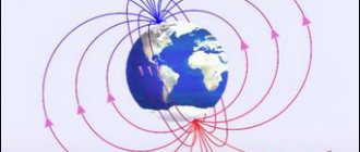
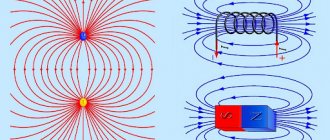
Everyone knows how magnets interact. They either attract or repel each other depending on the relative position of their poles, and this interaction occurs without direct contact of the magnets with each other. Therefore, it is believed that there is a special magnetic field around a magnet, different from the field of an electric charge. Then the interaction forces between magnets can be considered as a result of the interaction of their fields with the magnets themselves, i.e. the field of one magnet acts directly on another magnet, and vice versa. By analogy with the electric field, it is believed that there are lines of force in the magnetic field, especially since they are clearly distinguished by magnetic needles or iron filings (Fig. 1). Field lines indicate the direction of the magnetic field, which will be located tangent to the field line at any point. The direction of the magnetic field at a given point can be defined as the direction indicated by the north pole of a compass needle placed at that point, so the lines of force are always directed from the north pole of the magnet to the south. The magnetic field at any point in space can be represented by vector B, called magnetic induction, the magnitude of which can be determined through the torque acting on the magnetic needle when it is not oriented along the magnetic field line (Fig. 2). The greater the torque, the stronger the magnetic field. The magnetic needle will be in equilibrium when it is located tangent to the field line at a given location. The magnitude of the magnetic field is characterized by the density of field lines, i.e., their number per unit area. However, the physical essence of the magnetic field, like the electric field, remains unknown, and the induction vector B is determined experimentally. For this reason, there is obviously no theory of the interaction of permanent magnets and, surprisingly, there is not even experimental data on this interaction. And this can be understood, because without a theory, it is impossible to analyze the results of experiments. This section studies the interaction of permanent magnets using kinetic energy fields that exist around and inside the magnets and represent the vortex movement of vacuum particles created by the ordered movement of electrons in the magnet. The nature of the magnetic field, which is the vortex motion of vacuum, from the ends and cylindrical surface of the magnet is shown in Figure 3, and if you look at the magnet from its north pole, the rotation of the vacuum will occur clockwise, and if you look at it from the south pole, counterclockwise . This direction of rotation of vacuum particles corresponds to all experiments carried out with magnets. This will be shown below using a number of other examples of magnetic interactions. In a magnetic field, several areas can be distinguished for the purpose of their mathematical description: truncated cones at the ends (from the poles) and part from the side of the cylindrical surface. The angle at the tops of the poles is assumed to be equal to 900. An approximate diagram of the distribution of linear velocities of vacuum particles from the side of the cylindrical surface of the magnet is also shown here. It should be noted that this character of the magnetic field was chosen quite arbitrarily on the basis of the pattern of the so-called lines of force formed by the iron filings. The physical essence of this picture will be shown below. When studying the interaction of magnets from the poles, we will assume that only conical regions of magnetic fields interact. For any cross section of the cone, the angular velocity of vacuum rotation will be considered constant, depending only on the Z coordinate (Fig. 4): , (1) where R is the radius of the magnet, is the angular velocity of the vacuum on the end surface of the magnet, and is an unknown exponent. Let us prove the constancy of the angular velocity of the vacuum on the end surface of the magnet. Since the magnetic field is created by the rotation of electrons around the nucleus of an atom during their ordered movement throughout the entire volume of the magnet, the nature of the movement of the vacuum will depend on the result of the addition of the movements of vacuum particles under the influence of individual electrons. In Fig. Figure 5 shows the ordered movement of electrons around atomic nuclei at a certain distance r and r + 2r0 from the magnet axis, where r0 is the radius of the electron’s orbit. Since for a larger radius the number of electrons will be greater, the total circumferential speed of electrons for the outer atoms will be greater than for the inner layer of atoms. The difference between these speeds can be found through the number of atoms located on adjacent circles: ; (2) (3) The difference in the number of atoms on these circles is equal and, therefore, the uncompensated peripheral velocity will be equal to: , (4) where is the angular velocity of rotation of the electron around the atomic nucleus. Having accepted and , after integrating expression (4) we obtain: (5) Hence the angular velocity of vacuum rotation at any distance r from the magnet axis will be equal to: , (6) i.e. it will be constant and the same for the entire volume of the magnet, regardless of r. The peripheral speed of the vacuum particles will change according to a linear law depending on r. As for , expression (1) requires experimental verification. Expression (6) could be used to calculate the circular frequency of rotation of the magnetic field in the volume of the magnet if all electrons rotated in the same plane, i.e., the movement of all electrons would be ordered. However, this never happens, so the resulting rotation speed will be significantly less. For example, let's calculate the angular speed of rotation of an electron in a hydrogen atom, whose linear speed of rotation is approximately km/sec, and the distance to the nucleus is equal to m/s: This means that for a magnetic field this value will be less. Since there is no data on this matter, the circular frequency of rotation should be found from experiment. The truth is in [8, p. 74] for a proton nuclear resonance magnetometer, in which precession of nuclei occurring in a magnetic field occurs, the relationship between the precession frequency and the magnetic induction of field B, adopted by the MAGA Assembly in 1960, is given: This relationship can be taken as a starting point, but it is valid the ratio for solids (and not hydrogen, as in the device) should be less. Let us represent the circumferential velocity of vacuum in section Z by the expression (see Fig. 4): , (7) where the radius can be found from the relation (at , ): (8) from where: . (9) Then the peripheral speed will have the form: (10) where . Since the kinetic energy field arising during vacuum rotation will be non-uniform, a force due to the presence of a field gradient (force of inertia) will act on a particle of vacuum: , (11) where is the kinetic energy of the elementary mass, l is the coordinate characterizing the direction in space along which the derivative of the kinetic energy is taken. The kinetic energy of the elementary mass is determined by the expression: (12) Bearing in mind that and , after replacing the variable and differentiation, we reduce expression (11) to the following form: (13) where the coordinate l' is measured from the end surface of the magnet. The forces acting on all elementary masses will be summed up, as a result of which a force will act on the end surface of the magnet, the magnitude of which can be found by integrating expression (13) after substituting the expression for the elementary mass into it: (14) where , is the vacuum density. To find the axial resultant force, we use the projection of the elementary force onto the axis of the magnet: (15) As a result of integration, we obtain: (16) Obviously, exactly the same force will act on the other pole of the magnet, so the magnet will be in a balanced state. With the end interaction of the magnets, the equilibrium will be disrupted, since on the inside the volumes of the conical fields will be limited by the distance between the poles of the magnets (Fig. 6). When interacting with opposite poles, magnets will attract and like poles will repel. This nature of the interaction of magnets depends on the direction of the relative rotation of the vacuum in the cones of the magnets. With the same direction of vacuum rotation in interacting cones (from opposite poles), the forces acting on any magnet are determined by the fields of kinetic and potential energy, and it is assumed that the magnet’s own field is a field of kinetic energy, and the field of another magnet superimposed on it is a potential field energy. It is also believed that dynamic pressure does not arise in this case. When the vacuum rotates in different directions (like poles interact), it is assumed that the resulting kinetic energy field is determined by the difference between the own and superimposed kinetic energy fields. Accordingly, the potential energy field will be determined by the double value of the potential energy field. In this case, dynamic pressure arises, the magnitude of which will also be determined by double the potential energy. The forces determined by the potential energy field, as well as dynamic pressure, are taken with a negative sign. First, let's consider the interaction of magnets from opposite poles. To simplify the calculations, let’s take cylindrical magnets of the same size with the same induction B, i.e., with the same angular velocities on the end surfaces, since the mechanical analogue of induction can only be the circular frequency of vacuum motion. The value must be related to the induction B through an as yet unknown coefficient, where the coefficient has the dimension . The forces acting on the outer ends of the magnets will be determined by expression (16). On the inside, they are determined by the fields of kinetic and potential energy and , which for the cone of the first magnet will have the form: (17) (18) Let us present the velocities of vacuum particles for both magnets in accordance with expression (10) in the following form: ; (19) (20) where (21) (22) Bearing in mind that and using expressions (21) and (22), expression (20) is transformed to the form: (23) For the kinetic energy field, the axial force is determined by an expression similar to the expression (16), where the limits of integration over are taken in the range from 0 to: (24) The force from the potential energy field is determined by the expression (given without derivation, since it is done in a similar way, only the derivative over is taken with a negative sign): (25) (integral by l' in this expression will be taken below for the selected value of n). Thus, the magnet will be acted on by two forces from the inside, defined by expressions (24) and (25), and one force from the outside, defined by expression (16). Since the forces from the kinetic energy fields are directed in different directions, the resulting force will be equal to their difference and will press the magnets against each other. The magnitude of this force will be equal to: (26) The force from the potential energy field will repel the magnets. The total total force will press the magnets against each other. Let us now consider the interaction of magnet poles of the same name. The external forces acting on the magnets will remain the same, but the internal ones will change, since the rotation of the vacuum particles in the cones will occur in different directions and the energies of the particles will be subtracted. As a result of this, as noted above, the kinetic energy field in the cone will decrease, the potential energy field will increase by the same amount, i.e. it will double, and dynamic pressure will also appear. Thus, we will have: (27) (28) , (29) where is the dynamic pressure, dV is the volume of the elementary mass, determined by the ratio . Expression (29) characterizes the dynamic pressure on the end surface of the magnet (). The forces determined by the derivatives of kinetic and potential energy can be found using formulas (24) and (25), and formula (24) can be used without changes, and for formula (25) a factor of 3 should be introduced. The dynamic pressure force at the end the surface of the magnet can be found using the relations: ; (30) (31) The minus sign in expression (31) shows that the axial force from the dynamic pressure is directed towards the surface of the magnet. When deriving this formula, the following relation was used: . Thus, when like poles interact, two repulsive forces and one pressing force will act on the magnet. As a result, the magnets will repel each other. However, to use the resulting equations, it is necessary to know the exponent v and the circular frequency of rotation of the vacuum. In order to determine these values, the force of attraction between two identical cylindrical magnets with a diameter of 24 mm and a thickness of 8 mm was measured. The average induction value at the poles was 0.265 Tesla. The attractive force was determined for various values of L using a household dynamometer with a measurement limit of up to 10 kg. Then the equations were solved for various values of n (1; 1.5; 2; 2.5; 3). The best approximation to experimental data was obtained with v=3. Formula (25) in this case will be represented by the expression: (32) The theoretical curves for attraction and repulsion, as well as experimental results, are presented in Figure 7. As can be seen from the figure, the theoretical values of attraction and repulsion are not equal to each other, and the force of attraction is less. At v=2.5 the force of attraction will be greater than the force of repulsion. The force values will obviously be close in the range of 2.5
(47) where =11.810-15, as well as for the case of interaction of magnets with end fields. It is interesting to note that for any value the attractive force is not equal to the repulsive force. It also seems interesting to consider the interaction of magnets on the side of the poles during their relative tangential motion (at a constant distance between the poles). To simplify the problem, we will assume that their end magnetic fields have a cylindrical shape with a magnet radius R and with the same angular velocity in any section. Then the interaction of the fields will begin from the moment they touch when the magnets move in the tangential direction. From the point of view of the peculiarities of the interaction of fields, three characteristic mutual positions of magnets can be distinguished (Fig. 12, 13, 14), at which their interaxial distance lies respectively within the following limits: 1) ; 2) ; 3) . For each of these provisions there will be corresponding formulas for calculating the interaction. Let's consider the first case of interaction (Fig. 12). A feature of this interaction of magnets is that the fields partially overlap each other, and in relation to the interface, the fields will mutually change from the main one (kinetic energy field) to additional (potential energy field), i.e. the larger field will be considered the main one , less is additional. So, for example, for the first disk, its field will be the main one to the right of the partition border (right segment), and to the left of the border it will be additional (left segment). When the fields interact, the kinetic energy fields of the magnets will be subtracted, and the potential energy field will double if the angle between the velocities of the vacuum particles is greater than 900. If the angle is less than 900, the kinetic energy fields do not change, and the smaller field becomes the potential energy field. In both cases, we did not take into account the dynamic pressure, since it is not clear on which surface it should act. When the vacuum rotates in one direction for the left segment, the kinetic and potential energies are determined by the expressions: (48) (49) We accept where Then we get: (50) (51) Accordingly, the elementary forces will be equal: ; (52) (53) and their sum is determined by the expression: (54) Bearing in mind that , where h is the length of the magnet (since the forces will act on the microparticles of the magnet), we find the projection onto l of the total resulting force: (55) where . The factor 2 is introduced in (55) and subsequent expressions due to the symmetry of the forces acting on the two halves of the circle: from 0 to 1800 and from 1800 to 3600. For the right segment, the kinetic and potential energies will be equal: (56) (57) Forces, determined by these energies will respectively be equal to: (58) (59) (60) (61) where the Resultant force acting on both sections will be determined by the sum of the forces and . When rotating the vacuum in different directions, for the left segment we will have: (62) (63) (64) (65) (66) (67) where . For the right segment it will be: (68) (69) (70) (71) (72) (73) where . It should be noted that the integrals in the above formulas are easy to take, however, due to the large volume, these expressions are not given. With the second relative position of the magnets (Fig. 13), four sections can be distinguished both to the right of the dividing line (right segment) and to the left of it (left segment). Therefore, when rotating the vacuum in one direction for the left segment, we obtain: Section I: (74) ; (75) (76) (77) (78) (79) where . Section II: the force will be determined in general terms by the same expression as , only the limits of integration will be different: . III section: (80) (81) (82) (83) (84) (85) where IV section: the force is determined by expression (85) with the limits of integration: . For the right segment we will have: I section: (86) (87) (88) (89) (90) (91) where II section: the force is determined by expression (91) with the limits of integration: III section: (92) (93) (94) (95) (96) (97) where IV section: the force is determined by expression (97) with the limits of integration: . As a result, the total force acting on the first magnet will be the sum of eight forces. When rotating the vacuum in different directions for the left segment, we obtain: Section I: (98) (99) (100) (101) (102) (103) where Section II: the force is determined by expression (103) with the limits of integration: Section III: ( 104) (105) (106) (107) (108) (109) where IV section: the force is determined by expression (109) with integration limits: For the right segment we will have: I section: (110) (111) (112) ( 113) (114) (115) where II section: the force is determined by the expression (115) with the limits of integration: III section: (116) (117) (118) (119) (120) (121) where IV section: the force is determined by the expression (121) with integration limits: As a result, the force acting on the magnet from the two segments is determined by the sum of eight forces. At the third relative position of the magnets (Fig. 14), the left segment of the interacting fields is divided into five parts, and the right into three parts. When rotating the vacuum in one direction for the left segment, we obtain: Section I: (122) (123) (124) (125) (126) (127) where Section II: the force is determined by expression (127) with the limits of integration: Section III: ( 128) (129) (130) (131) (132) (133) where IV section: force is determined by expression (133) with integration limits: V section: force is also determined by expression (133) with integration limits: . For the right segment we will have: I section: (134) (135) (136) (137) (138) (139) where II section: (140)
(141) (142) (143) (144) (145) where III section: the force is determined by the expression (145) with the limits of integration: The total resulting force acting on the first magnet from the two field segments will be equal to the sum of eight forces. For all considered cases of field interaction, calculations were made, the results of which are presented in Figure 15. What is unexpected is the change in the sign of the interaction force when the relative distance changes, both when rotating in one direction and the other. However, this phenomenon makes it possible to explain the braking of a magnetic pendulum in the field of another magnet. Let us consider the oscillations of a cylindrical magnet with a diameter of 2R on a suspension of length l in the field of another cylindrical magnet of the same diameter (Fig. 16). To simplify the calculations, we assume that the force of interaction between magnets appears when the cylindrical fields overlap each other, i.e., starting from a distance of 2R between the axes, and we present the law of change of magnetic force in an approximate form: , (146) where is the amplitude value of the force, is the current value angle of rotation, is the angle of deflection of the pendulum corresponding to the distance 2R. In Fig. Figure 16 shows the diagram and zone of action of this force, and in the first half-wave the magnetic force will be repulsive. We will also assume that in all positions the magnetic force is directed tangentially to the trajectory of the magnet. The amplitude value of the force is determined by the formula: , (147) where for these magnets =0.1; ; 1/s; R=m; m; kg/m3, where FН. comes from! The pendulum will also be affected by the gravity force of the magnet G, equal to 0.3 N. The equation of motion of the pendulum in general is characterized by the equation: , (148) where J is the moment of inertia of the pendulum relative to the suspension point, the moment of all forces acting on the pendulum. The movement of the pendulum can be divided into two sections: 1) only under the influence of gravity from corner to corner; 2) under the influence of gravity and force from an angle to a vertical position. Then we get: 1) for the first section: ; (149) 2) for the second section: (150) The minus sign in front of the moment is placed because the argument, when changing from to 0, changes from to 0 in the negative direction, i.e., clockwise. In the first section, the pendulum, under the influence of gravity, accelerates to a certain speed, the value of which is determined by the expression [3, p.572]: (151) under initial conditions: ; . There is no solution to equation (150) in general form. Therefore, for the purpose of an approximate analysis of motion, we will not take into account the moment from the weight, since it is significantly less than the moment from the magnetic force. Then, introducing a new variable (152) and taking into account the initial conditions: ; (153) , (154) we find the angular velocity of the pendulum in the second section: , (155) where (156) Moving on to the original notation, we obtain: (157) To determine the angular speeds of the pendulum in both sections, we set the length of the pendulum l = 0.1 m and initial deflection angle . Having accepted that , where m = 0.03 kg and having found rad = 13.750 using formula (151), we determine: 1/s Then we find the value of the angle at which the speed will be equal to zero, for which we equate to zero the expression under the root in formula (157 ), from which we obtain: (158) Substituting the values of all quantities included in this expression, we determine: , from which and . Thus, for this case of interaction of magnets, the pendulum will slow down when it reaches an angle of 0.840, i.e. won't do even one full swing. Obviously, a similar braking mechanism will operate due to induction when using a copper plate instead of a stationary magnet. In conclusion, let us consider the issue of the so-called magnetic lines of force, which clearly appear before us in the form of a certain picture of iron filings. Since this picture is an objective reality, it should characterize some features of the movement of vacuum around a magnet. It is generally accepted that magnetic forces are directed tangentially to the lines of force. But will it really be like this? If particles of iron filings are considered as small magnets (magnetic arrows), their position will be determined by the forces of interaction of the fields of the magnets with the field of the magnet. The interaction of a magnetic needle with a vacuum flow can be considered (by analogy with a solid body) by adding the velocities inside the volume of the magnet itself (see Fig. 17, a). The magnitude of the interaction force is determined by the expression: , (159) where is the mass of the vacuum in the volume of the magnet; — angular velocity of vacuum rotation in the magnet; is the linear velocity of vacuum particles in the magnetic field at a distance . In Fig. Figure 17a shows the direction of the force F arising from the interaction of fields inside the magnet, and this force will be directed against the gradient of the total field. In Fig. 17,a the following notations are adopted: , where is the radius of the magnet (the magnet is considered as a cylinder); — instantaneous center of velocities of the total field. In Fig. Figure 17, b shows the initial position of the magnet, the center of which is located at a distance Z from the surface of the magnet, and the magnet itself is located in the direction of the radius vector. With this position of the magnet, a greater force will act on its lower half, and a lesser force on the upper half. Under the influence of a greater force, the magnet will begin to rotate clockwise (for this case) until the forces are equalized, which can only happen if the velocities of the vacuum particles in the external magnetic field are equal. Indeed, when the magnet is rotated, the velocities of the vacuum particles will be equalized, since the near end of the magnet will move away from the magnet and approach the axis, and the far end will approach the magnet and move away from the axis. With distance from the surface of the magnet, the vacuum speed decreases, and with increasing radius, it increases. Let us derive calculation formulas for the angle of rotation of the magnet. From the geometric relationships we obtain: ; (160) ; (161) ; (162) , (163) where is the length of the magnet. From here we will have: ; (164) ; (165) Since , expressions (164) and (165) are transformed into the form (dividing the numerator and denominator by R): (166) (167) The linear velocities of particles at the extreme points of the magnet are determined by the expressions (see formula (10)): ; (168) ; (169) where Equating these speeds, we obtain the relation: (170) Expressions (166), (167) and (170) are used as follows. First, they are set by the values , , , i.e., the size of the magnet and the coordinates of its center. Then, using the selection method, angle values are found that satisfy these expressions for the selected value of n. In Fig. Figure 18 shows the position of the magnets from the end part of the magnet we studied at and n=3. As can be seen from the figure, the pattern of the location of the magnets is generally similar to the pattern of the location of iron filings. From this we can conclude that the filings or magnetic needles are located not in the direction of the lines of force, but along the lines of equal velocities of the vacuum particles rotating around the magnet. These lines should be called isotachs. And one more interesting circumstance should be noted: the iron filings are arranged in such a way that they form clear lines that do not touch each other. This obviously gave reason to talk about magnetic lines of force. The explanation for this phenomenon is quite simple: iron filings, like small magnets, cannot come into contact with each other, since they all rotate the vacuum in the same direction and interact with cylindrical surfaces by repulsion, as shown above. Using the picture of the arrangement of iron filings around the magnet, one can find the value of the exponent v, which characterizes the decrease in the linear velocity of the vacuum with distance from the magnet. Thus, having transformed expression (170), we obtain a formula for the experimental determination of v on the end side of the magnet (from the side of the poles): (171) This formula will be valid at a constant angular velocity of rotation of the vacuum within the cone for any cross section Z. However, such the assumption may not actually be fulfilled, then formula (171) will be approximate. There is also another independent experimental method for determining the exponent v by measuring the magnetic field induction at various distances from the surface of the magnet. The location of the sensor for two measurements of magnetic induction from the end of the magnet is shown in Fig. 19. Since during the interaction of magnets it was assumed that induction was proportional to the angular velocity of vacuum rotation, obviously, induction will be proportional to the linear velocity of vacuum particles if the sensor is located at the same distance from the magnet axis. In this case, the following relations can be written: ; (172) , (173) where B is the induction on the surface of the magnet; and are the radii on the surface of the magnet corresponding to the two positions of the sensor; and are the coordinates of the sensor center. The radii and can be found from the relationships (see Fig. 19): ; (174) ; (175) Substituting these ratios into expressions (172) and (173) and dividing the first by the second, we obtain: , (176) from where, after logarithmization, we find the exponent v: (177) For the magnet we studied, the induction at distances = 1 mm and = 6 mm, respectively, was equal to =0.265 T and =0.155 T. At R=12 mm, the value of v will be equal to: , i.e., it coincides quite well with the value of v found from the force interaction. After determining v, you can find the value of induction directly on the surface of the magnet using one of the formulas (172) or (173), for example: , (178) from which for our case we will have: Thus, summing up all of the above, we can say that the expected the hypothesis of the interaction of permanent magnets through a material vacuum, despite the accepted assumptions, explains quite well the nature of magnetism, the reasons for the emergence of forces of attraction and repulsion at different mutual positions of the magnets, the reason for the braking of the magnetic pendulum and the physical essence of magnetic lines of force.
Here is a brief derivation of relation (22): whence (22) follows.
How do magnets attract and repel?
How are magnets attracted? A force arises between magnets brought close to each other. The attraction or repulsion of magnets is felt not only during direct contact. There is interaction even without contact.
Magnets will repel each other if their north poles are brought close to each other. When the south poles contact, a similar picture will be observed. However, attraction will arise between the magnets if the south pole is brought close to the north pole. This principle works similarly to electric charges. In this case, the poles of magnets and electric charges are different phenomena.
Bottom line
Neodymium magnets are products that are widely used in various commercial, industrial and domestic applications. This material has a high load-carrying capacity, as well as excellent attractive properties and a long service life.
Before demagnetizing a neodymium magnet, you need to make sure that you have all the necessary equipment for this process. To perform this process properly, you need to use special industrial equipment or a device capable of generating heating up to eighty degrees above zero.
If the product has lost its own qualities, then the process associated with the magnetization of this material is rarely performed, since this is an impractical solution. But, when it is most necessary, you can order such a process by contacting the manufacturer.
For what reason are not all materials capable of magnetization?
A magnet interacts with a wide range of substances. The type of interaction is not limited to attraction or repulsion. Certain metals and alloys have a specific structure, which makes it possible to be attracted to a magnet with a certain power.
Other materials also have this property, but on a smaller scale. To detect attraction under such conditions, it is necessary to create a very strong magnetic field. This is not possible at home. Why do all materials have the property of attraction, but only metal can be perceived as magnetic? The answer lies in the special external structure of atoms.
The things around us are made up of atoms connected to each other. The type of connection between them determines the material. The atoms in most substances are poorly grouped, so the bond with the magnet is weak. In a metal, atoms are well coordinated; all atoms synchronously sense the magnetic field and are drawn towards it.
Nature and principle of action
Permanent magnets are natural substances and precision alloys with significant residual magnetization that lasts for a long time.
They are made from ferromagnetic materials - substances that can maintain magnetization in the absence of a magnetic field; they are found in a number of minerals (ores). Substances susceptible to the influence of magnets include: iron, cobalt, nickel. An alloy of iron and cobalt has higher ferromagnetic properties than each metal separately. Electrons moving in an atom due to rotation form tiny vortex magnetic fields. The basis of the magnetic field is created by an atom rotating around its own axis, like planets, their satellites, and stars.
Why are some materials not attracted to a permanent magnet, but others “stick” perfectly? It's a matter of direction, orientation of magnetic lines. In non-magnetic materials (substances with extremely weak magnetization), the fields of atoms are directed in different directions, often canceling each other rather than strengthening them.
In a number of metals, atoms are structured and combined into groups - domains - miniature magnets. At rest, a piece of steel does not have magnetic properties, and the field applied to it orders these domains; they are oriented in one direction, the lines of force add up.