- Equations and graphs
- Rationale for vector diagram
- Effective value of alternating current
Sinusoidal emf. and current:
The receipt, transmission and use of electrical energy is carried out mainly using alternating current devices and structures. For this purpose, generators, transformers, transmission lines and AC distribution networks are used. The most widely used electrical energy receivers are those operating on alternating current. Alternating electric current is an electric current that changes over time (see Fig. 2.1, curves 2, 3).
A periodic electric current that is a sinusoidal function of time is called a sinusoidal electric current.
In practice, this current is usually meant when talking about alternating current. In some cases, the current varies according to a periodic non-sinusoidal law.
In linear electrical circuits, alternating sinusoidal current arises under the influence of e. d.s. the same shape. Therefore, to study electrical devices and alternating current circuits, it is necessary to first consider methods for obtaining sinusoidal e. d.s. and basic concepts related to quantities that vary sinusoidally.
Obtaining sinusoidal emf.
To get e. d.s. An industrial-type sinusoidal alternating current generator has certain design features. However, the fundamentally sinusoidal dependence of e. d.s. versus time can be obtained by rotating a conductor in the form of a rectangular frame at a constant frequency in a uniform magnetic field (Fig. 12.1).
Rice. 12.1. Rectangular frame in a magnetic field
Rotation of a coil in a uniform magnetic field
According to formula (10.5), e. d.s. in a frame having two active conductors of length l,
With uniform rotation of the frame, the linear speed of the conductor does not change: and the angle between the direction of the speed and the direction of the magnetic field changes in proportion to time: Angle β determines the position of the rotating frame relative to the plane perpendicular to the direction of magnetic induction. (The position of the frame at the start of time t = 0 is characterized by the angle β = 0.) Therefore, e. d.s. in the box is a sinusoidal function of time. The greatest value of e. d.s. reaches at angle In the case considered, the sinusoidal change in e. d.s. is achieved by continuously changing the angle at which the conductors intersect the lines of magnetic induction. However, this method of obtaining e. d.s. is not used in practice, since it is difficult to create a uniform field in a sufficiently large volume.
Alternator
In electric machine alternating current generators of industrial type, sinusoidal e. d.s. obtained at a constant angle, but in a non-uniform magnetic field.
The magnetic field of the generator (radial) in the air gap between the stator and the rotor is directed along the radii of the rotor circle (Fig. 12.2, a). Magnetic induction along the air gap is distributed according to a law close to sinusoidal. This distribution is achieved by the appropriate shape of the pole pieces. The sinusoidal distribution law of magnetic induction along the air gap is shown in Fig. 12.2, b in expanded form.
Rice. 12.2. Alternator circuit diagram. Distribution of magnetic induction along the air gap
Rice. 12.3. Circuit diagram of an alternator with two pairs of poles on the rotor
Rice. 12.4. Generator circuit with three turns (windings)
At any point in the air gap, the position of which is determined by the angle β measured from the neutral plane (neutral) counterclockwise, the magnetic induction is expressed by the equation
The neutral plane is perpendicular to the axis of the poles and divides the magnetic system into symmetrical parts, one of which belongs to the north pole, and the other to the south.
The magnetic induction has the greatest value under the middle of the poles, i.e. at angles and At the neutral (at β = 0 and β = 180°), the magnetic induction is zero (B = 0). In Fig. Figure 12.3 shows the design diagram of an alternating current generator with two pairs of poles located on the rotor, and the conductors of the winding where the electricity is induced. d.s., placed in the grooves of the stator core.
Let us note another type of alternating current generators - a generator with three windings (three-phase generator), which in the diagram in Fig. 12.4 are represented by three turns on the rotor (for turbogenerators and hydrogenerators, these windings are located on the stator). The planes of the turns are at an angle of 120° to each other.
E.D.S. in the generator winding
With uniform rotation of the rotor in its winding (in Fig. 12.2, a - in a coil), e.m. is induced. d.s., determined by formula (10.4). Substituting the expression for magnetic induction (12.3), we obtain
At β = 90°, i.e. in the position of the conductor under the middle of the pole, the greatest e is induced. d.s. Equation e. d.s. can be written as follows: Taking into account formula (12.1), we obtain the same dependence of the emf. from time, as when rotating the frame (see Fig. 12.1), considering the initial position of the coil (t = 0), when its plane coincides with the neutral: Thus, in this case, e. d.s. is a sinusoidal function of time (Fig. 12.5). The same result is obtained if the poles are rotated and the conductors are left motionless.
Rice. 12.5. Graph of sinusoidal e. d.s.
In a rectangular coordinate system, e. d.s. can be represented as a function of angle or as a function of time t. The dependence and can be depicted by one curve, but with different scales along the abscissa axis, differing by ω times. If the generator winding is closed through a resistance, then a sinusoidal current appears in the resulting circuit, repeating the shape of the e curve. d.s. Assuming the circuit resistance to be linear, equal to R, we obtain the following expression for the current: where is the largest current value. Sinusoidal voltage and current can be obtained using generators that do not have rotating parts and magnetic poles, such as tube generators.
Problem 12.1.
E.m.f. electric machine generator is expressed by the equation. Determine the number of pole pairs of this generator if the rotor speed n = 75 rpm is known. At what angle in space does the generator rotor rotate during 1/4 of a period? Solution. Period e. d.s., induced in the winding of a generator (see Fig. 12.2), which has one pair of poles, is equal to the time of full rotation of the rotor. The angular speed of rotation of the rotor can be determined by the ratio of the total angle corresponding to one revolution of the rotor to the period: However, the generator may have not one, but p pairs of poles (in Fig. 12.3 p = 2). Full cycle of change e. d.s. in this case, it occurs when the conductor moves past one pair of poles (as during a full revolution of the rotor in a generator with p = 1), therefore, at the same rotor speed, the emf period With. will be p times shorter, and the frequency will be p times greater. A decrease in period and a corresponding increase in frequency for a given number of pole pairs can be obtained by increasing the rotor speed. Frequency of sinusoidal e. d.s. at p = 1 it is equal to the number of rotor revolutions per second, and at p > 1 where n is the rotor speed, rpm. From Eq. d.s. the angular frequency ω = 314 rad/s is known; while at rotor speed n = 75 rpm
At p = 1, in 1/4 of the period the rotor will rotate 1/4 of the circle, i.e., angularly by 90º. At p = 40, the angle of rotation of the rotor for 1/4 of the period will be p times less:
Addition and subtraction of vectors
Figure 12, a shows three vectors A, B and C. Figure 12, b shows their addition according to the parallelogram rule, namely: first, the sum of two vectors A and B (B and C, A and C) is found, and then to vector C (A, B) is added to it. Figure 12c shows another way of adding these same vectors in four options. Pay attention to the direction of the sum vector. Comparing Figures 12, b and c, it is easy to see that in any case the same results were obtained.
Figure 12. Addition and subtraction of vectors
To subtract one vector from another, the subtracted vector is rotated 180° (that is, it is given the opposite sign), after which addition is performed according to the parallelogram rule (Figure 12, d). Another way to subtract the same vectors is illustrated in Figure 12, d. Note: the difference vector is directed towards the end of the vector from which the subtraction was made. So, in Figure 12, d, on the left, the difference vector is directed towards the end of vector B.
Equations and graphs of sinusoidal quantities
It is impossible to analyze AC electrical circuits without expressing e. d.s. currents, voltages and their equations. For clarity, graphs of these quantities in a rectangular coordinate system are used. Therefore, let's look at the equations and graphs of sinusoidal quantities in more detail.
Equations and graphs
Equation (12.4) is written for the case when the beginning of the time count (t = 0) coincides with the moment the coil passes through the neutral (in Fig. 12.2, a is position 1, in which the plane of the coil coincides with the neutral).
In Fig. 12.4, the position of the turns also corresponds to the beginning of the time count (t = 0) and is determined for each of them by an angle measured from the neutral to the plane of the turn: for the first turn, this angle for the second - and third - When the rotor rotates, e. d.s. will be induced in all turns, but the emf equations will not be the same. Indeed, at = 0 e. d.s. in turns: This dependence e. d.s. from the initial position of the coil is taken into account by introducing the initial angle into the equation. Taking into account the initial angle e. d.s. turn C is expressed by the equation
e. d.s. turn B
Thus, in general form, the equation e. d.s. should be written like this:
From this equation you can determine the value of e. d.s. at any moment at an arbitrary initial position of the coil. In Fig. 12.6, in accordance with equation (12.6), graphs of the emf of three turns are plotted, differing at the start of the time count by their location relative to the neutral plane (eA at eC at eB at ).
Rice. 12.6. Graphs e. d.s., phase shifted
Characteristics of sinusoidal quantities
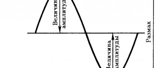
The equation and graph specify all the characteristics of a sinusoidally varying quantity: amplitude, angular frequency, initial phase, period, frequency, and instantaneous value for any moment in time.
The following are definitions of these characteristics and they are shown in Fig. 12.7 in relation to sinusoidal e. d.s. The definitions apply to all quantities that vary according to a sinusoidal law (current, voltage, etc.).
Rice. 12.7. On the question of the characteristics of periodic e. d.s.
Instantaneous value (or instantaneous value) e. d.s. e is the value of e. d.s. at the moment in time under consideration. Instant e. d.s. is determined by equation (12.6) by substituting into it the time t that has passed from the beginning of the countdown to a given moment.
Period T is the shortest time interval after which the instantaneous values of the periodic e. d.s.. are repeated. If the argument of the sine function is expressed in angles, then the period is expressed by the constant value 2π. Frequency f is the reciprocal of the period: that is, the frequency is equal to the number of periods of the variable e. d.s. per second. Frequency is expressed in hertz (Hz): 1 Hz = 1/s. Amplitude Em is the largest value that e takes. d.s. during the period. Amplitude is one of the instantaneous quantities that corresponds to an argument equal to , where k is any integer or zero. Phase (phase angle) is the argument of the sinusoidal emf, measured from the nearest previous e.m. transition point. d.s. through zero to a positive value. The phase at any time determines the stage of the harmonic change of the sinusoidal e. d.s. The initial phase ψ is the phase of the sinusoidal emf. at the initial moment of time. Two sinusoidal quantities having different initial phases are said to be out of phase. Angular frequency ω is the rate of phase change. During one period T, the phase angle uniformly changes by 2π, therefore
Problem 12.4.
Alternating electric current is given by the equation
Determine the period, frequency of this current and its instantaneous values at t = 0; t1 = 0.152 s. Draw a current graph. Solution. The sinusoidal current equation in the general case has the form Comparing this equation with the given partial current equation, we establish that the amplitude Im = 100 A, angular frequency ω = 628 rad/s, initial phase ψ = -60°. Period Frequency
Rice. 12.8. For Problem 12.4
We find the instantaneous current values by substituting the given time values into the current equation:
at t = 0 at t1 = 0.152 s The sinusoidal value is repeated after 360°, so the instantaneous current at the angle will be the same as at the angle: To construct a graph, you need to determine a series of instantaneous currents corresponding to different moments of time (Fig. 12.8).
How are sinusoids constructed?
Figure 3 shows how sinusoids are constructed. On the horizontal axis, either time is plotted, increasing from left to right, or the angles of rotation of the winding (magnet), which are counted from a certain position taken as the initial one. The values of e are plotted along the vertical axis. d.s., current or other periodic quantity, proportional to the sines of the rotation angles. Angles can be measured in degrees or radians. In Figure 3, time is given in fractions of a period: T/4, T/2, ¾ T, T; rotation angles are also shown: 0, 30, 60, 90, ..., 360°. It must be borne in mind that in bipolar generators the period corresponds to a full revolution, that is, it is completed through 360°, or 2π radians, that is, in order for one of the winding conductors, leaving under the north (south) pole, to return to it, it must rotate 360°. Therefore, in Figure 3, which is built for a two-pole generator, the period T corresponds to 360°, the half period T/2 to 180°, the quarter period T/4 to 90°, and so on.
Figure 3. Technique for constructing a sine wave
In multi-pole generators, the electrical and geometric degrees do not coincide, because the poles of the same name, for example the north ones, are located closer to each other: in a four-pole generator at a distance of 180°, in a six-pole generator - at a distance of 120°, and so on. And since, regardless of the number of poles, all generators produce current of the same industrial frequency, that is, they have the same periods, the generator rotors must make different paths in the same time: a revolution, half a revolution, a third of a revolution, and so on. Therefore, generator rotors have different rotation speeds, that is, they rotate at different rotation frequencies (speeds): the fastest are two-pole (3000 rpm), four-pole ones make 1500 rpm, six-pole ones 1000 rpm, and so on.
Let us note one extremely important circumstance: the sinusoid is a periodic curve, that is, it has neither end nor beginning, and therefore it is not at all necessary to draw it starting from 0°. With equal success, you can start with 30, 47, 122 (-60°) and so on. But since in these cases the countdown will start later or earlier, it needs to end the same amount later or earlier.
Vector diagrams
Until now, quantities varying according to a sinusoidal law were specified by equations and depicted by graphs in a rectangular coordinate system. When calculating AC electrical circuits, they use a very simple and visual method of graphically representing sinusoidal quantities using rotating vectors.
Rationale for vector diagram
Let us assume that the current is given by the equation Let us draw two mutually perpendicular axes and from the point of intersection of the axes we draw the vector Im, the length of which on a certain scale Mi expresses the amplitude of the current Im:
Rice. 12.10. On the issue of vector diagram
We choose the direction of the vector so that with the positive direction of the horizontal axis the vector makes an angle equal to the initial phase ψ (Fig. 12.10).
The projection of this vector onto the vertical axis determines the instantaneous current at the initial moment of time: Let us imagine that the vector Im rotates counterclockwise with an angular velocity equal to the angular frequency ω. Its position at any moment of time is determined by the angle. Then the instantaneous current for an arbitrary moment of time t can be determined by the projection of the vector Im onto the vertical axis at this moment in time. For example, for t = t1 in the general case, we obtained the same equation as the alternating current was specified, which indicates the possibility of depicting the current as a rotating vector when applied to the drawing: in the initial position.
Construction of a vector diagram
By rotating the vector Im' counterclockwise, in a rectangular coordinate system we will construct a graph of changes in its projection onto the vertical axis within one revolution (one period). We obtain the already known graph of the sinusoidal function corresponding to the given equation.
When constructing vectors, positive angles are counted from the positive direction of the horizontal axis counterclockwise, and negative angles are counted along its movement.
In the process of calculating an electrical circuit, a number of sinusoidal quantities are determined. All of them can be depicted on one drawing using rotating vectors, tied to one pair of mutually perpendicular axes.
A set of vectors depicting in one drawing several sinusoidal quantities of the same frequency at the initial moment of time is called a vector diagram. For example, voltage and current in an electrical circuit are expressed by the equations
The vector diagram of such a circuit is shown in Fig. 12.11. If you choose the voltage and current scales then
Rice. 12.11. Vector diagram of current and voltage
A vector diagram contains vectors of sinusoidal quantities of the same frequency, so they rotate with the same frequency and their relative positions do not change.
The time reference point is chosen arbitrarily, so one of the diagram vectors can be directed arbitrarily; the rest must be positioned taking into account the phase shift relative to the first or previous vector.
Addition and subtraction of vectors
The simplicity and clarity of vector diagrams is not the only and not the main advantage of the method of depicting sinusoidal quantities. It is required to add, for example, two currents given by equations. The expression for the sum turns out to be cumbersome, and the amplitude and initial phase of the resulting current are not visible from it.
You can graphically add two given currents, plotting them in one coordinate system and for a number of arguments, finding the sum of two ordinates. We draw a sum curve through the obtained points and see that this curve is also a sinusoid with the same period as the terms. From the total current curve you can find the amplitude and initial phase. The bulkiness and inconvenience of such an addition are obvious.
It is very simple to add and subtract sinusoidal quantities using the rules for adding and subtracting vectors.
Rice. 12.12. Vector addition
Let's add two given currents i1 and i1 according to the well-known rule of vector addition (Fig. 12.12, a). To do this, we depict the currents in the form of vectors from a common origin 0. We find the resulting vector as the diagonal of a parallelogram built on the terms of the vectors:
It is more convenient to add vectors, especially three or more, in this order: one vector remains in place, the others are transferred parallel to themselves so that the beginning of the next vector coincides with the end of the previous one. Vector Im, drawn from the beginning of the first vector to the end of the last, is the sum of all vectors (Fig. 12.12, b).
Subtraction of one vector from another is performed by adding the forward vector - the minuend and the reverse - the subtrahend (Fig. 12.13):
Rice. 12.13. Vector subtraction
Rice. 12.14. Special cases of vector addition
When adding sinusoidal quantities, in some cases an analytical solution can be applied: in relation to Fig. 12.12, a - according to the cosine theorem; to fig. 12.14, a - addition of vector modules; b - subtraction of vector modules, c - according to the Pythagorean theorem.
Problem 12.7. The two currents are given by the equations
Find the current equations: Solution. The easiest way to solve a problem is graphically in vector form. To do this, let us depict the vectors of the given currents. We select the current scale so that the largest vector fits on an existing sheet of paper, while at the same time taking into account the possibility of a clear image of the smallest vector. When analyzing the solution, it is recommended to construct according to Fig. 12.15 on a sheet of graph paper on a scale. On this scale, the length of the vectors
The length of the sum vector is determined graphically (Fig. 12.15, a):
Rice. 12.15. For Problem 12.7
The initial phase of this vector according to the drawing Equation of the sum of currents In the same order, the vectors of current differences were found (Fig. 12.15, b, c). The subtracted vectors are taken in antiphase with the given ones. After measuring the lengths of the vectors and initial phases, we will write the equations for the current differences:
Phase
It was already indicated above that the windings of generators, transformers and electric motors are called phases. But the word “phase” in electrical engineering is used in several other meanings.
Phases are also called wires of three-phase lines, in contrast to the neutral wire. The phases are designated by the letters A, B, C (a, b, c) or Ж, З, К, since in power plants and substations buses belonging to different phases are painted with yellow, green and red paints. Zero is denoted by the number 0, and sometimes by the letter N (neutral).
A phase in the broad sense of the word is a separate moment in the development of a phenomenon. In periodic processes (which include changes in emf and current), the phase is the value of a quantity that characterizes the state of the oscillatory process at each moment of time.
Thus, the phase can be called both the angle of rotation of the winding (since each angle corresponds to a certain emf value) and the time elapsed from the beginning of the period. The beginning of the period when e. d.s. equal to zero, often called zero phase.
Phase angles that determine the values of e. d.s. or current at the initial moment (from which the consideration of the process of changing emf or current begins), are called initial phases .
It is important to understand that when determining the phase shift between two e. d.s. or currents, it must always be determined between identical phases of the quantities under consideration. For example, the shift α between zero phases (Figure 7, a) and between phases in T/5 (Figure 7, b) is the same.
Figure 7. Determination of the phase shift value
If you need to determine whether one sinusoid is ahead of another or behind it, proceed as follows.
Through the zero phase 01 of one sinusoid (ax), a vertical 1–1 is drawn until it intersects with the second sinusoid (by) (Figure 8, a). If the vertical intersects the sinusoid above the horizontal axis, then the second sinusoid is ahead of the first; if lower, it lags behind . Indeed, the vertical 1–1, drawn through the zero phase of the sinusoid ax, intersects by above the horizontal axis and, therefore, by is ahead of ax. But if by is ahead of ax, then ax is behind by. This can be easily verified by drawing vertical 2–2 (Figure 8, b) through the zero phase by, which intersects the lagging sinusoid ax below the horizontal axis.
Figure 8. Determining the direction of phase shift
Effective and average values of alternating current
Everything is known about alternating current if its equation or graph is given. However, in practice it is difficult to use equations or current graphs. Alternating current is usually characterized by its effective value I. When studying rectifier devices and electrical machines, average values of e are used. d.s., current, voltage.
Effective value of alternating current
When determining the effective value of alternating current, one can proceed from any of its actions in the electrical circuit (thermal, mechanical interaction of wires with currents).
In Fig. Figure 12.18 shows graphs of two currents: constant 1 and alternating 2, and the magnitude of the direct current is equal to the amplitude of the alternating current. A direct current equal to the amplitude of an alternating current will release more heat in the same circuit element at the same time, since the alternating current is less than constant during a half-cycle, and only for one instant these currents are equal.
The effective magnitude of the alternating current I is numerically equal to the magnitude of the direct current, which in the same circuit element during the period T emits the same amount of heat as the alternating current emits under the same conditions.
The effective magnitude of the alternating current I is less than the amplitude (straight line 3 in Fig. 12.18).
Rice. 12.18. To determine the effective value of alternating current
Let us determine the amount of heat generated over a period T by a direct current equal to I and an alternating current (see Fig. 12.18) in a circuit element with resistance R: By equating we find
The effective value of the periodic current is its root mean square for the period.
It can be found from equation (12.9), but for clarity we will use a graphical solution to the problem.
The root mean square value of the alternating current over a period can be represented as the square root of the sum of a very large number of ordinates of the curve i2(t), divided by the number of ordinates n: where the numerator of the radical expression represents the sum of the squares of a number of instantaneous currents during the period, n is the number of these values , tending to ∞. In Fig. Figure 12.19 shows a number of positions of the current vector Im rotating at an angular speed ω and the corresponding instantaneous currents i. These positions are marked by points 0, 1, 2, etc. on the circle that the end of the vector Im describes.
Let us consider two positions of the vector Im (marked by points 2 and 8), separated by 90° along the circle, i.e., located in the first and second quarters of the circle, respectively. Right triangles 6′-2-2′ and 6′-8-8′ are equal because their sides are equal: 2-2′ = 6′-8′ and 2′-6′ = 8-8′. From these triangles it follows:
Rice. 12.19. To determine the effective and average value of the sinusoidal current
Each position of the vector Im in the first quarter corresponds to its other position in the second, for which a similar expression can be written. Such reasoning can be carried out for another semicircle, i.e., extend it to the second half-cycle of the current, and the squares of the negative instantaneous currents will be positive, therefore, substituting this expression in (12.10), we obtain Thus, the effective value of the sinusoidal current is less than its amplitude by a factor.
The concept of effective magnitude can be extended to all sinusoidal functions and, therefore, we can talk about the effective magnitude of voltage, e. d.s.
Effective values of current and voltage are measured by electrical measuring instruments. Rated currents and voltages of electrical devices are expressed in effective quantities. Having introduced the concept of effective magnitude, in the future we will construct vector diagrams for effective quantities of voltages and currents.
The ratio of the amplitude to the effective value is called the amplitude coefficient Ka. For a sinusoidal function this coefficient is equal to ; if the current or voltage curve has a sharper shape than a sinusoid, then Ka > , otherwise Ka (with a rectangular shape Ka = 1).
Adding and subtracting sinusoids
In electrical installations in which several electrical currents operate. d.s., depending on the method of connection, they can either be added or subtracted. The same applies to currents at branching points.
In DC , addition and subtraction are performed algebraically. This means that if one e. d.s. is 5 V, and the other is 18 V, then their sum is 5 + 18 = 23 V, and the difference is 5 – 18 = –13 V. The minus sign indicates a change in the direction of the current in the opposite direction compared to that which would be from only one e. d.s. 5 V.
In AC , addition and subtraction are more complex.
To add two sinusoids e1 and e2 you need to: a) intersect them in several places with verticals 0, 1, 2, 3, 4, 5 ... and so on, at which the sinusoids will cut off the instantaneous values of e. d.s. (Figure 11, a); b) pairwise algebraically add the instantaneous values and the resulting sums, which are the instantaneous values of the total e. d.s., set aside on the same verticals (Figure 11,b); c) connect the vertices of the total instantaneous values with a smooth curve, thus obtaining a total sinusoid from another, for example e1 + e2.
Figure 11. Addition and subtraction of sinusoids
To subtract one sinusoid from another, for example e1 from e2 (Figure 11, a), you need to give the subtracted sinusoid the opposite sign, that is, simply draw its mirror image –e1 (Figure 11, c). Then sinusoids e2 and –e1 are added (Figure 11, d), as described above. In a word, subtraction of sinusoids is based on the well-known rule, which states that subtracting is the same as adding the same thing with the opposite sign.