Representation of sinusoidal currents and voltages by rotating vectors on the complex plane and in complex form. Vector diagrams of currents and voltages.

Vector diagrams and complex representation

Vector diagrams can be considered a variant (and illustration) of representing oscillations as complex numbers. With this comparison, the Ox axis corresponds to the axis of real numbers, and the Oy axis corresponds to the axis of purely imaginary numbers (the positive unit vector along which is the imaginary unit).

Then a vector of length A

, rotating in a complex plane with a constant angular velocity
ω
with an initial angle
φ0
will be written as a complex number

and its real part

-there is a harmonic oscillation with a cyclic frequency ω

and the initial phase
φ0
.

Although, as can be seen from the above, vector diagrams and a complex representation of oscillations are closely related and essentially represent variants or different sides of the same method, they nevertheless have their own characteristics and can be used separately.

• The method of vector diagrams can be presented separately in courses in electrical engineering or elementary physics if, for one reason or another (usually related to the moderate level of mathematical preparation of students and lack of time), it is necessary to avoid the use of complex numbers (explicitly) at all.

• The complex presentation method (which, if necessary or desired, can also include a graphical presentation, which, however, is completely unnecessary and sometimes unnecessary) is generally more powerful, because naturally includes, for example, the compilation and solution of systems of equations of any complexity, while the method of vector diagrams in its pure form is still limited to tasks involving summation, which can be depicted in one drawing.

• However, the method of vector diagrams (in its pure form or as a graphical component of the complex representation method) is more visual, and therefore, in some cases, potentially more reliable (allows, to some extent, to avoid gross random errors that can occur in abstract algebraic calculations) and allows In some cases, to achieve, in some sense, a deeper understanding of the problem.

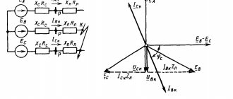
Calculation formulas for a circuit with parallel connections of branches. Vector diagram method

From the vector diagram it is clear that all the active components of the current vectors are directed in the same way - parallel to the voltage vector, so their vector addition can be replaced with arithmetic to find the active component of the total current: Ia = I1a + I2a + I3a .

The reactive components of the current vectors are perpendicular to the voltage vector, with inductive currents directed in one direction, and capacitive ones in the other. Therefore, the reactive component of the total current in the circuit is determined by their algebraic sum, in which inductive currents are considered positive and capacitive currents are considered negative: Ip = - I1p + I2p - I4p + I5p .

The active, reactive and total current vectors of the entire circuit form a right triangle, from which it follows

Substituting the magnitudes of currents in the branches, expressed in terms of voltage and corresponding conductivities, we obtain

where ∑Gn is the total active conductivity , equal to the arithmetic sum of the active conductivities of all branches ; ∑Bn is the total reactive conductivity, equal to the algebraic sum of the reactive conductivities of all branches (in this sum, inductive conductivities are considered positive, and capacitive conductances are considered negative); Y is the total conductivity of the circuit;

In this way, the already familiar formula (14.12) is obtained, connecting voltage, current and conductivity of the circuit [cf. (14.12) and (14.8)].

Attention should be paid to possible errors when determining the total conductivity of a circuit from the known conductivities of individual branches: it is impossible to add arithmetically the conductivities of the branches if the currents in them are out of phase.

The total conductivity of a circuit is generally defined as the hypotenuse of a right triangle, the legs of which are the active and reactive conductivities of the entire circuit expressed on a certain scale:

From the current triangle you can also go to the power triangle and to determine the power you can obtain the already known formulas

The active power of a circuit can be represented as the arithmetic sum of the active powers of the branches.

The reactive power of the circuit is equal to the algebraic sum of the powers of the branches. In this case, the inductive power is taken to be positive, and the capacitive power to be negative:

Types of vector diagrams

Vector graphics are well suited for correctly displaying variables that determine the functionality of radio devices. This implies a corresponding change in the basic parameters of the signal along a standard sinusoidal (cosine) curve. To visualize the process, harmonic oscillation is represented as a projection of a vector onto the coordinate axis.

Using standard formulas, it is easy to calculate the length, which will be equal to the amplitude at a certain point in time. The tilt angle will indicate the phase. The total influences and corresponding changes in vectors obey the usual rules of geometry.

There are high-quality and accurate diagrams. The first ones are used to take into account mutual connections. They help make a preliminary assessment or are used to completely replace calculations. Others create taking into account the results obtained, which determine the size and direction of individual vectors.

Pie chart

Let us assume that we need to study the change in current parameters in a circuit for different values ​​of resistor resistance in the range from zero to infinity. In this circuit, the output voltage (U) will be equal to the sum of the values ​​(UR and UL) on each of the elements. The inductive nature of the second quantity implies a perpendicular relative position, which is clearly visible in part of figure b). The triangles formed fit perfectly into the 180 degree circle segment. This curve corresponds to all possible points through which the end of the vector UR passes with a corresponding change in electrical resistance. The second diagram c) shows a current lag in phase by an angle of 90°.

Line chart

Shown here is a two-pole element with active and reactive conductivity components (G and jB, respectively). A classic oscillatory circuit created using a parallel circuit has similar parameters. The parameters noted above can be represented by vectors that are constantly located at an angle of 90°. A change in the reactive component is accompanied by a movement of the current vector (I1...I3). The formed line is located perpendicular to U and at a distance Ia from the zero point of the coordinate axis.

Mechanics; harmonic oscillator

• A harmonic oscillator in mechanics and a harmonic oscillator of any nature formally represent an exact analogy, so we will consider them in one paragraph using the example of a mechanical harmonic oscillator.
• The use of vector diagrams in mechanics is reduced mainly to the case of a harmonic oscillator (including the case of an oscillator with a friction force linear in speed); however, vector diagrams can be to some extent useful for studying several oscillators, including in the limit of an infinite number of them (for oscillations or waves in distributed systems).
• From a modern point of view, the application of vector diagrams to a harmonic oscillator is rather of only historical and pedagogical interest, but nevertheless, in principle, they are quite applicable here.
• In mechanics, the use of vector diagrams (usually meaning their application to a one-dimensional oscillator) has the peculiarity that the addition of a second coordinate to transform oscillations into rotation can have not only a purely formal abstract meaning, but for a one-dimensional mechanical system of this kind a mechanical two-dimensional system can be indicated , for which the vector diagram is the first to be realized as a completely real two-dimensional mechanical movement, and all vectors are really two-dimensional (and after projecting all of them and moving a point of a two-dimensional system onto one axis, we obtain instantaneous values ​​of the corresponding quantities - including positions - for the corresponding one-dimensional system ); Thus, for a mechanical one-dimensional system, not only a formal mathematical, but also a real mechanical
  model is possible, transforming oscillatory one-dimensional motion into rotational motion in two-dimensional space, implementing a vector diagram for a one-dimensional system.

Let us examine two main cases of simple application of vector diagrams in mechanics (as noted above, also applicable to a harmonic oscillator not only of mechanical, but of any nature): an oscillator without damping and without external force and an oscillator with (linear) damping (viscosity) and external forcing by force.

Representation of sine functions as complex numbers

A vector diagram is a convenient tool for representing sinusoidal functions of time, which are, for example, voltages and currents of an alternating current electrical circuit.

Consider, for example, an arbitrary current represented as a sine function

i(t) = 10 sin(ωt + 30°).

This sinusoidal signal can be represented as a complex quantity

I = 10∠30°.

To form a complex number, the magnitude and phase of the sinusoidal signal are used.

Vector diagram for series connection of elements

To construct vector diagrams, first compose equations according to Kirchhoff's laws for the electrical circuit in question.

Let's consider the electrical circuit shown in Fig. 1, and draw a vector voltage diagram for it. Let us denote the voltage drop across the elements.

Rice. 1. Series connection of circuit elements

Let's create an equation for this chain according to Kirchhoff's second law:

UR + UL + UC = E.

According to Ohm's law, the voltage drop across the elements is determined by the following expressions:

UR = I ∙ R,

UL = I ∙ jXL,

UC = −I ∙ jXC.

To construct a vector diagram, it is necessary to display the terms given in the equation on the complex plane. Typically, current and voltage vectors are displayed on their own scales: separately for voltages and separately for currents.

From the mathematics course we know that j = 1∠90°, −j = 1∠−90°. Hence, when constructing a vector diagram, multiplying a vector by an imaginary unit j results in a rotation of this vector by 90 degrees counterclockwise, and multiplication by −j results in a rotation of this vector by 90 degrees clockwise.

When constructing a vector diagram of voltages on the complex plane, we will first display the current vector I, after which we will display the voltage drop vectors relative to it (Fig. 2), taking into account the above relations for the imaginary unit.

The voltage drop across the resistor UR coincides in direction with the current I (since UR = I ∙ R, and R is a purely real value or, in simple words, there is no multiplication by an imaginary unit). The voltage drop across the inductive reactance leads the current vector by 90° (since UL = I ∙ jXL, and multiplying by j leads to a rotation of this vector by 90° counterclockwise). The voltage drop across the capacitive reactance lags behind the current vector by 90° (since UC = −I ∙ jXC, and multiplying by −j leads to a rotation of this vector by 90° clockwise).

Rice. 2. Vector diagram of voltages for a series connection of circuit elements. Please note that one vector diagram shows only the vectors of those quantities whose frequency coincides!

Vector diagram for parallel connection of elements

Let's consider the electrical circuit shown in Fig. 3, and draw a vector diagram of currents for it. Let us denote the direction of the currents in the branches.

Rice. 3. Parallel connection of circuit elements

Let's create an equation for this chain according to Kirchhoff's first law:

I – IR – IL – IC = 0,

where

I = IR + IL + IC.

Let us determine the currents in the branches according to Ohm’s law using the following expressions, taking into account that 1 / j = −j:

IR = E/R,

IL = E / (jXL) = −j ∙ E / XL,

IC = E / (−jXC) = j ∙ E / XC,

To construct a vector diagram, it is necessary to display the terms given in the equation on the complex plane.

When constructing a vector diagram of currents on the complex plane, we will first display the EMF vector E, after which we will display the current vectors relative to it (Fig. 4), taking into account the above relations for the imaginary unit.

The current in the resistor IR coincides in direction with the emf E (since IR = E / R, and R is a purely real quantity or, in simple words, there is no multiplication by an imaginary unit). The current in the inductive reactance lags behind the EMF vector by 90° (since IL = −j ∙ E / XL, and multiplying by −j results in a rotation of this vector by 90° clockwise). The current in the capacitive reactance leads the EMF vector by 90° (since IC = j ∙ E / XC, and multiplying by j leads to a rotation of this vector by 90° counterclockwise). The resulting current vector is determined after the geometric addition of all vectors according to the parallelogram rule.

Rice. 4. Vector diagram of currents for parallel connection of circuit elements

For an arbitrary circuit, the algorithm for constructing vector diagrams is similar to the above, taking into account the currents flowing in the branches and the applied voltages.

Please note that the site provides a tool for constructing vector diagrams online for three-phase circuits.

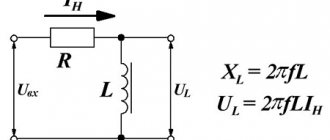
Circuit with resistor and inductor

An alternating current circuit with these two elements connected in series is shown in Figure 4.6, a.

The voltage applied to the coil consists of two terms: the voltage drop in the active resistance Ua = Ir and the inductive resistance Ul = I ∙ xL.

Since the voltage drop vector Ua coincides in direction with the current vector, and the vector UL is ahead of it by 90°, then by adding both vectors geometrically, we obtain the voltage vector U (Figure 4.6, b). Thus, in a circuit with a real coil, the current also lags behind the voltage, but by an angle φ less than 90°.

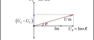
Triangle AOB is called the voltage triangle of an alternating current circuit containing active and inductive resistance.

The following relationships follow from the stress triangle:

The projection of the voltage vector onto the current vector is called the active component of the voltage vector and is denoted Ua, and the projection of the voltage vector into the direction perpendicular to the current vector is called the reactive component of the voltage vector and is denoted Up. By analogy, the current vector can be decomposed into active and reactive components:

Figure 4.7 - Electric circuit with a resistor, inductor and capacitor: a) - circuit; b) - vector diagram of voltage and current

If the sides of the voltage triangle are divided by the current I, we obtain a resistance triangle (Figure 4.6, c), the legs of which are active r and inductive xL resistance, and the hypotenuse is the value z =, called the total resistance of the circuit.

The circuit current is determined by Ohm's law:

The phase shift angle between current and voltage is determined from vector diagrams (Figure 4.6, b, c):

or

4.7 Circuit with resistor, inductor and capacitor

Figure 4.7 a shows an alternating current electrical circuit with active resistance (resistor), inductance (coil) and capacitance (capacitor).

In such a circuit, the effective value of the applied voltage consists of three components: active Ua, inductive UL and capacitive UC: U = Ua + UL + UC (the summation is done geometrically, Figure 4.7, b).

Individual components of effective voltage values:

From the vector diagram it can be seen that the active voltage drop Ua coincides with the current, the inductive UL leads the current by 90°, and the capacitive UC lags the current by 90°.

From the voltage triangle OAS it follows that the voltage applied to the circuit:

Hence the current:

This formula expresses Ohm's law as applied to an unbranched alternating current circuit.

The phase shift between voltage and current is determined by the expression:

Circuit resistance, determined by the formula:

Called the impedance of the circuit. Resistance x = xL - xC is called reactive.

The following cases of ratios xL and xC are possible:

· xL > xC then φ > 0, inductance predominates in the circuit;

· xL < xC, then φ < 0, capacitance prevails in the circuit;

· xL = xC, or ω ∙ L = l/ω ∙ C, then φ = 0, cos φ = 1.

The circuit resistance is minimal, while the current reaches the highest possible value. The voltage at the coil and capacitor terminals can exceed the voltage at the circuit terminals by tens of times. Therefore, resonance when elements are connected in series is called voltage resonance. Voltage resonance can only occur with small active circuit resistances. The voltage resonance mode in high current technology is an emergency, since in this case the insulation of the capacitor coils can be broken. In high-frequency technology (radio engineering), voltage resonance is a normal mode and is used to amplify voltages.

At the angular frequency w of the supplied voltage, voltage resonance can be obtained by changing the capacitance C or the inductance of the circuit L so that ω ∙ L = 1/ω ∙ C, or with constant L and C of the circuit - by changing the frequency of the supplied voltage.

The angular frequency of natural oscillations in the circuit is ωо = 1/ or frequency f = 1/2 ∙ π ∙ , i.e. ωо ∙ L = 1/ ω ∙ C. Consequently, the phenomenon of resonance occurs when the frequencies of the oscillatory circuit and the alternating current source are equal ωо = ω. The angular frequency ωо at which resonance occurs is called the resonant angular frequency of the circuit and depends only on the magnitude of the inductance and capacitance of the circuit.

Figure 4.8 - Electric circuit with parallel connection of a resistor, inductor and capacitor: a) - diagram; b) and c) - vector diagrams of voltage and current; d)id) - conductivity triangles

With voltage resonance, the energy of the magnetic field Wm = L ∙ I2/2 is equal to the energy of the electric field We = C ∙ U2/2 and is transferred from the coil to the capacitor and back with fluctuations in current and voltage without consuming energy from the source. Undamped oscillations arise. Energy is exchanged between the coil and the capacitor through an energy source that replenishes the energy lost in active resistances.

4.8 Parallel connection of resistor, inductor and capacitor

In such a circuit (Figure 4.8, a), the effective value of the current in the unbranched part of the circuit consists of three terms: active Ia, inductive IL and capacitive IC:

(the summation is done geometrically).

The following cases of relationships between IC and IL are possible: current IC > IL then φ < 0, the current in the unbranched part of the circuit leads the voltage; vector Iр (segment AC), indicating the reactive component of the current, is directed upward from the voltage vector (Figure 4.8, b); current IC < IL, then φ > 0, the current in the unbranched part of the circuit lags behind the voltage, the vector Iр (segment AC) is directed downward from the voltage vector (Figure 4.8, c); current IC = IL, then φ = 0; cos φ = 1, the current in the unbranched part of the circuit is in phase with the voltage and is equal to the active current, i.e. I = Ia.

The active component of the current Ia has the same sign for any values ​​of φ. The reactive component of the current changes sign along with the change in the sign of the angle φ. Dividing each side of the current triangle by the effective voltage U, we obtain a conductivity triangle (Figure 4.8, d, e).

Since cos φ = r/z, a sin φ = x/z, we obtain expressions for currents and conductivities for an equivalent parallel connection:

where g = - active conductivity;

b = bL - bc = xL/z2 - xC/z2 = x/z2 - reactive conductivity;

y = = is total conductivity.

From the conductivity triangle:

Effective current value in the unbranched part of the circuit:

If a branched circuit consists of inductance and capacitance connected in parallel, then in such a circuit, with the equality ω ∙ L = 1/ω ∙ C, the phenomenon of current resonance occurs, in which the currents in the branches IL and IC (Figure 4.8, a) are equal to each other and can significantly exceed the total current I flowing in the unbranched part of the circuit.

The conditions for the appearance of current resonance are similar to the conditions for the appearance of voltage resonance.

With current resonance, all the energy supplied to the circuit is spent on heat generation in the active resistance of the circuit, and an oscillatory exchange of stored energy occurs between the inductance and the capacitance.

The current resonance mode is of great practical importance. Electrical resonant circuits are used in radio engineering, measuring technology, telecontrol, and various automation circuits. Resonance phenomena are also used to change the parameters of power lines. By connecting capacitors in parallel to an active-inductive load, the load power factors are increased, relieving electrical networks from reactive power flows.

Power, energy (work)

In DC circuits, power consumption is defined as the product of voltage and current, energy (work) - as the product of power and time. In AC circuits, in most cases such a simple calculation is not possible.

If the alternating current circuit contains only active resistance, without inductive and capacitive resistance, then the active power is defined as the product of the effective values ​​of voltage and current P = U ∙ I or P = I2 ∙r. This power is spent in active resistance and does useful work.

Usually in an alternating current circuit, along with active resistance, there is also inductive and often capacitive reactance. In such circuits there is a phase shift between current and voltage, therefore the active power developed by the current is less than the product U ∙ I, i.e. P = U ∙ I cos φ.

The units of active power, like DC power, are: watt (W), kilowatt (kW), megawatt (MW).

The value of cos φ is called the power factor of the AC circuit. The larger this coefficient, i.e., the smaller the phase shift angle between current and voltage, the greater the active power of the circuit at the same values ​​of current and voltage. Therefore, the active power reaches its greatest value in circuits with purely active resistance (φ = 0, cosφ = 1), and in circuits with purely inductive resistance the active power is zero (φ = 90°, cosφ = 0).

Electrical energy Wa consumed in an alternating current circuit during time t is defined as the product of active power and time and is active energy:

.

Figure 4.9 — Vector power diagram (power triangle)

Active energy is measured in kilowatt-hours (kW∙h) and its consumption is recorded by active energy meters. The alternating current circuit is also characterized by reactive Q and apparent power S. Reactive power Q = U ∙ I sin φ. It is a measure of the rate of energy exchange between the current source and the consumer. Without performing useful work, it serves only to create magnetic fields in inductive receivers (electric motors, transformers), circulating all the time between the current source and the receivers of electrical energy. The unit of reactive power is the reactive volt-ampere (var). The larger unit is 1 kilovolt-ampere reactive (kvar); 1 kvar = 103 var. The product of reactive power Q and time t is called reactive energy W ∙ P = Q ∙ t = U ∙ I ∙ t ∙ sin φ.

Reactive energy is measured in kilovar-hours (kvar ∙ h). Reactive energy is metered using reactive energy meters.

Total power S = U ∙ I is the maximum possible active power in the absence of phase shift (φ = 0, cos φ = 1). Apparent power is measured in volt-amperes (V ∙ A) or kilovolt-amperes (kV ∙ A). It is the main parameter characterizing alternating current generators and power transformers.

Total, active and reactive powers are related to each other by the ratio:

or

Those. the same ratio as the sides of a right triangle, the legs of which represent active and reactive power, and the hypotenuse - the total power of the circuit (Figure 4.9).

From the power triangle it follows that:

Active power:

Reactive power:

Algorithm for creating a ray vector diagram in Excel

To simplify our lesson, let's assume that we are talking about relationships not between fourteen as in the graph, but for now only with 4 people named Anton, Alice, Boris and Bella.

Our matrix of the level of relationships and connections between them looks like this:

• 0 means no relationship;
• 1 means weak relationship (for example: Anton and Alice just know each other);
• 2 means a strong relationship (for example, Boris and Alisa are friends).

How can we geometrically model the visualization of this raw data? If we were to draw the relationship between these four people (Anton, Alice, Boris and Bella), it would schematically look like this:

2 criteria that we need to determine:

1. Location of dots (where people's names are printed).
2. Lines (starting and ending points of connecting lines).

Defining and plotting points

First we need to plot our points so that the space between each point is the same. This will create a balanced schedule.

Which geometric figure best satisfies our need for such equal intervals? Of course it's a circle!

You might object that the finished diagram model does not have a circle shape. Yes, really no - that's it. We don't need to draw a circle. We just need to plot the points around it.

So we have 4 stakeholders, we need 4 points:

1. If we have 12 stakeholders, we need 12 points.
2. If we have 20, we need 20 points.

Assuming the origin of our circle is (x, y), the radius is r and theta is 360 divided by the number of points we need. The first point (x1, y1) on the circle will be at this position:

• x1 = x + r * COS (theta);
• y1 = y + r * SIN (theta).

Once all the points are calculated and connected to the XY chart (scatter plot), let's move on.

Drawing lines on a ray diagram

Let's say we have n people in our network. This means that each person can have a maximum of n-1 relationships.

Thus, the total number of possible lines on our graph is n * (n-1) / 2.

We need to divide it by 2, as if A knows B, then B also knows A. But we only need to draw 1 line.

The network graph analysis ray diagram template is configured to work with 20 people. It can be downloaded at the end of the article and used as a ready-made analytical tool for visualizing these connections. This means that the maximum number of rows we can have will be 190.

Each line requires adding a separate series to the chart. This means we need to add 190 series of data for just 20 people. And it only satisfies one line type (dashed or thick). If we want different lines depending on the type of relationship, we need to add another 190 episodes.

It's painful and funny at the same time. Fortunately, there is a way out!

We can use a much smaller number of series and still produce the same graph.

Let's say we have 4 people - A, B, C and D. For the sake of simplicity, let's assume that the coordinates of these 4 people are as follows:

• A – (0.0);
• B – (0.1);
• C – (1,1);
• D – (1.0).

And let's say A has relationships with B, C and D.

This means that we need to draw 3 lines, from A to B, from A to C and A to D.

Now, instead of putting 3 series for the chart, what if we put one long series that looks like this:

(0,0), (0,1), (0,0), (1,1), (0,0), (1,0)

This means we simply draw one long line from A to B, A to C, A to D. Granted, it's not a straight line, but Excel scatter plots can draw any line if you give it a set of coordinates.

See this illustration to understand the technique:

So instead of 190 series of data for the chart, we just need 20 series.

In the last chart we have 40 + 2 + 1 series of data. It's because:

• 20 lines for weak relationships (dashed lines);
• 20 lines for strong relationships (thick lines);
• 1 line for highlighting in blue the weak relationships of the selected participant;
• 1 line for highlighting in green the strong relationships of the selected participant;
• 1 set without lines, but just dots for data labels on the graph.

How to generate all 20 data series:

This requires the following logic:

• Assuming we need lines for person n's relationships.
• This person's point will be (Xn, Yn) and has already been calculated earlier (at points on the graph around the circle).
• We only need 40 rows of data.
• Every odd row will have (Xn, Yn).
• For each even row:
• divide the line number by 2 to get the person's number (say m>);
• (Xn, Yn) if there is no relationship between n and m>;
• (Xm, Ym) if there are relations.

We need MOD and INDEX formulas to express this logic in Excel.

Once all line coordinates have been calculated, add them to our scatter plot as new series using the tool from the additional menu: “WORKING WITH DIAGRAMS” - “CONSTRUCTOR” - “Select data” in the “Select data source” window, use the “Add” button to adding all 43 rows.

We will implement the creation of such a ray diagram of connections in 3 stages:

1. Preparation of initial data.
2. Data processing.
3. Visualization.

Preparing data for a ray diagram

As mentioned above, this template will have the ability to visually build connections for up to 20 participants (companies, branches, counterparties, etc.). The template worksheet "Data" provides a table for populating incoming values. For example, let’s fill it out for 14 market participants:

On the same sheet we will create an additional table, which is a matrix of connections of all possible participants, generated by the formula:

With the data preparation completed, we move on to processing.

How to calculate the sum of vectors?

Vectors and matrices in a spreadsheet are stored as arrays.

It is known that the sum of vectors is a vector whose coordinates are equal to the sums of the corresponding coordinates of the original vectors:

To calculate the sum of vectors you need to perform the following sequence of actions:

– Enter the values ​​of the numerical elements of each vector into ranges of cells of the same size.

– Select a range of cells for the calculated result of the same dimension as the original vectors.

– Enter the formula for multiplying ranges into the selected range

– = Vector_Address_1 + Vector_Address_2 Address

– Press the key combination [Ctrl] + [Shift] + [Enter].

Example.

Two vectors are given:

It is required to calculate the sum of these vectors.

Solution:

– To cells in the range A2:A4

Let's enter the values ​​of the coordinates of vector a1, and into the cells of the range
C2:C4
- the coordinates of vector a2.

– Select the cells of the range in which the resulting vector C will be calculated ( E2:E4

) and enter the formula into the selected range:

=A2:A4+C2:C4

– Press the key combination [Ctrl] + [Shift] + [Enter]. In cells in the range E2:E4

the corresponding coordinates of the resulting vector will be calculated.

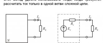
Calculation of a circuit without determining the conductivities of the branches

Calculation of an electrical circuit with a parallel connection of branches can be performed without first determining active and reactive conductivities , i.e., presenting the circuit elements in an equivalent circuit with active and reactive resistances (Fig. 14.15, a).

The currents in the branches are determined using formula (14.4);

where Z1, Z2 , etc. are the impedances of the branches.

The total resistance of a branch, which includes several elements connected in series, is determined by formula (14.5).

To construct a vector diagram of currents (Fig. 14.15, b), you can determine the active and reactive components of the current of each branch using the formulas

etc. for all branches.

In this case, there is no need to determine the angles φ1 φ2 and plot them in the drawing.

Current in the unbranched part of the circuit

The total current and power of the circuit are determined further in the same order as shown earlier (see formulas (14.10), (14.15), (14.16)].