Alternating current
(AC - Alternating Current) - an electric current that changes its magnitude and direction over time.
Often in the technical literature, a variable is a current that changes only the magnitude, but does not change the direction, for example, a pulsating current. It must be remembered when making calculations that alternating current in this case is only a component of the total current. This option can be represented as alternating current AC
with a constant
DC
. Or as direct current with an alternating component, depending on which component is most important in the context.
DC
- Direct Current - direct current that does not change its magnitude and direction.
In reality, direct current cannot maintain its value constant, therefore it exists conditionally in those cases where changes in its constant value can be neglected, or as a component ( DC
) for periodically changing electric current of any shape.
Then the DC
will be equal to the average current value for the period, and will be the zero line for the variable component
AC
.
With a sinusoidal current shape, for example in an electrical network, the DC
equal to zero.
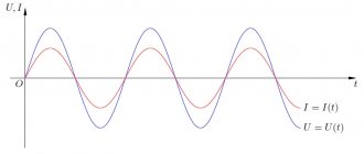
Direct current with an alternating component in the form of ripples is shown by the blue line in the upper graph of the figure. AC+DC recording
in this case it is not a mathematical sum, but only indicates two components of the current.
The powers are summed up. The current value will be equal to the square root of the sum of the squares of two quantities - the value of the constant component DC
and the root mean square value of the variable component
AC
.
AC terms
and
DC
are applicable for both current and voltage.
AC current and voltage parameters
The magnitude of alternating current, like voltage, constantly changes over time. Quantitative indicators for measurements and calculations use their following parameters:
Period
T
is the time during which one complete cycle of current change occurs in both directions relative to zero or the average value.
Frequency
f
is the reciprocal of the period, equal to the number of periods in one second.
One cycle per second is one hertz (1 Hz). Frequency f =
1
/T
Cyclic frequency
ω
- angular frequency equal to the number of periods in
2π
seconds.
ω = 2πf = 2π/T
Typically used in sinusoidal current and voltage calculations. Then, within the period, one can not consider frequency and time, but make calculations in radians or degrees. T = 2π = 360°
The initial phase
ψ
is the value of the angle from zero (
ωt
= 0) to the beginning of the period. Measured in radians or degrees. Shown in the figure for the blue sinusoidal current graph.
The initial phase can be a positive or negative value, respectively to the right or left of zero on the graph.
Instantaneous value
- the magnitude of voltage or current measured relative to zero at any selected time
t
.
i = i(t); u = u(t)
The sequence of all instantaneous values in any time interval can be considered as a function of the change in current or voltage over time. For example, a sinusoidal current or voltage can be expressed by the function:
i = Iampsin(ωt); u = Uampsin(ωt)
Taking into account the initial phase:
i = Iampsin(ωt + ψ); u = Uampsin(ωt + ψ)
Here Iamp
and
Uamp
are the amplitude values of current and voltage.
Amplitude value
— maximum modulo instantaneous value for the period.
Iamp = max|i(t)|; Uamp = max|u(t)|
Can be positive or negative depending on its position relative to zero. Often, instead of the amplitude value, the term amplitude
current (voltage) - maximum deviation from zero value.
Average value
(avg) - defined as the arithmetic mean of all instantaneous values over the
period T.
The average value is a constant component of DC
voltage and current. For sinusoidal current (voltage), the average value is zero.
Average rectified value
— arithmetic mean of the modules of all instantaneous values for the period.
For a sinusoidal current or voltage, the rectified average value is equal to the arithmetic mean over the positive half-cycle.
Root Mean Square (rms) - Defined as the square root of the arithmetic mean of the squares of all instantaneous values over a period.
For sinusoidal current and voltage amplitude Iamp
(
Uamp
) root mean square value is determined from the calculation:
Root mean square is the current, effective value, most convenient for practical measurements and calculations. It is an objective quantitative indicator for any form of current. In an active load, the alternating current does the same work during the period as a direct current equal in magnitude to its root-mean-square value.
Special cases of current amplitude values
In the event that the circuit consists only of active resistance $(R)$, then:
the current coincides with the voltage in phase, the amplitude of the current in this case is equal to:
Are you an expert in this subject area? We invite you to become the author of the Directory Working Conditions
If we compare equation (6) with expression (3), we can conclude that if, instead of a capacitor, a section of the circuit is simply short-circuited, this will mean a transition to a capacitance equal to infinity.
Let the resistance $(R=0)$ be neglected in the circuit, and the capacitance be considered equal to infinity, then:
The quantity $X_L$ is called inductive reactance (inductive reactance) if it is equal to:
From the formula it follows that the inductance does not resist direct current (at $\omega$=0, $X_L$=0).
Let us assume that $R=0,\ L=0.$ Then, according to formula (3), we obtain:
The quantity $X_C=\frac{1}{\omega C}$ is called reactance capacitance (capacitance) . If the current is constant, then $X_C=\infty $. This means that no direct current flows through the capacitor.
In the event that R=0, the amplitude of the current is equal to:
Reactance (reactance) $(X)$ is a value equal to:
Parameters of sinusoidal electrical quantities
Sinusoidal EMF, voltages and currents can be depicted graphically in the form of corresponding sinusoids; such graphs in electrical engineering are called wave diagrams (see Fig. 13).
Typically, one wave diagram depicts several sinusoids of variable quantities (voltages, currents) related to the same circuit. To assess their relative position along the abscissa axis, the difference in their initial phases, called the phase shift, is introduced. The most common phase shift occurs between current and voltage.
Wave diagrams are not always convenient for research, especially with complex branched circuits. In this case, it is easier to represent sinusoidal quantities with rotating vectors. Let us depict a rotating vector corresponding to the current:
Any vector on the plane drawn from the origin and depicting the value of emf, voltage or current is uniquely determined by the point corresponding to the end of this vector (point in the figure).
A complex number (corresponding to a point) has real (OS) and imaginary (IV) components on the complex plane.
Alternating (sinusoidal) current and the main quantities characterizing it.
Alternating current (AC) - electric current
, which changes in magnitude and direction over time or, in a particular case, changes in magnitude while maintaining its direction in the electrical circuit unchanged.
In everyday life, alternating, sinusoidal current is used for power supply.
Sinusoidal current is a current that changes over time according to a sinusoidal law (Figure 1):
The maximum value of the function is called amplitude. It is denoted using a capital (capital) letter and a lowercase letter m - the maximum value. Eg:
Period T is the time it takes to complete one complete oscillation.
f = 1/T
ω = 2πf = 2π/T
The argument of the sine, i.e. ( ωt + Ψ ), is called the phase . The phase characterizes the state of oscillation (numerical value) at a given time t.
Any sinusoidally varying function is determined by three quantities: amplitude, angular frequency ( ω ) and initial phase Ψ (psi)
In the CIS countries and Western Europe, sinusoidal current installations with a frequency of 50 Hz, accepted as standard in the energy sector, are most widespread. In the US, the standard frequency is 60 Hz. The frequency range of practically used sinusoidal currents is very wide: from fractions of a hertz, for example in geological exploration, to billions of hertz in radio engineering.
Sinusoidal currents and EMF of relatively low frequencies (up to several kilohertz) are obtained using synchronous generators (they are studied in the course of electrical machines). Sinusoidal currents and EMF of high frequencies are obtained using tube or semiconductor generators (discussed in detail in the radio engineering course and in less detail in the TOE course). A source of sinusoidal EMF and a source of sinusoidal current are designated on electrical diagrams in the same way as sources of constant EMF and current, but they are designated e and j (or e(t) and j(t)).
Source
Average voltage
The average value of the alternating voltage Uav is, roughly speaking, the area under the oscillogram relative to zero over a certain period of time. To understand this, let's look at this oscillogram.
average voltage value for the period
For example, what is the average voltage value for these two half-cycles? In this case, zero volts . Why is that? The areas of S1 and S2 are equal. But the whole point is that the area S2 is taken with a minus sign. And since the areas are equal, they add up to zero: S1+(-S2)=S1-S2=0. For an infinite time sinusoidal signal, the average voltage value is also zero.
The same applies to other signals, for example, a bipolar meander. A square wave is a rectangular signal in which the pause and pulse durations are equal. In this case, its average voltage will also be zero.
meander
Average rectified voltage value
Most often, the average rectified voltage value Uav is used. vypr. That is, the signal area that “breaks through the floor” is taken not with a negative sign, but with a positive one.
the average rectified voltage value will no longer be equal to zero, but S1+S2=2S1=2S2. Here we summarize the areas, regardless of which one they are familiar with.
In practice, the average rectified voltage value is easy to obtain by using a diode bridge. After rectifying the sinusoidal signal, the graph will look like this:
rectified AC voltage after the diode bridge
In order to find out approximately what the average rectified voltage is equal to, it is enough to find out the maximum amplitude of the sinusoidal signal Umax and calculate it using the formula:
Parameters of sinusoidal electrical quantities
Periodic emfs, voltages and currents are widely used in electrical circuits of electrical, radio and other installations. Periodic quantities change over time ( i=i(t); u=u(t)
) in value and direction, and these changes are repeated at some equal time intervals T, called a period (Fig. 13).
The most widespread are currents that vary according to a sinusoidal (harmonic) law.
Sinusoidal current is characterized by the following parameters:
In European countries, f = 50 Hz is accepted as the standard industrial frequency; in the USA and Japan, f = 60 Hz.
The difference in the initial phases of two sinusoidal quantities of the same frequency ( ) is called the phase shift between them:
Sinusoidal current has a number of advantages over direct current, and therefore it has become very widespread:
a) it is easy to transform from one voltage to another,
b) when transmitting over long distances (hundreds and thousands of kilometers) from source to consumer with multiple transformations, the voltage remains unchanged, i.e. sinusoidal,
c) with its help, a rotating magnetic field used in synchronous and asynchronous machines can be quite simply obtained.
To quantify sinusoidal functions of time, the concepts of effective and average values are introduced. The effective value of a sinusoidal current is the magnitude of such a direct current that has an equivalent thermal effect. Effective values are designated I,U,E,P
Similarly for voltage and EMF
The vast majority of instruments measuring sinusoidal currents and voltages are calibrated in effective values.
The average value of sinusoidal current or voltage and EMF is called the average for a half-period of time:
The amplitude values of sinusoidal quantities are designated: Im, Um, Em, Pm
Source
RMS voltage
Most often, the root mean square voltage value , or it is also called effective . In the literature it is simply designated by the letter U. To calculate it, you can’t get away with a simple graph. The rms value is the value of a direct voltage that, passing through a load (say, an incandescent lamp), releases in the same period of time the same amount of power as an alternating voltage will release in this load. In English, root mean square voltage is denoted as follows: RMS (rms) - root mean square.
The relationship between the amplitude and root mean square value is established through the amplitude coefficient Ka :
Ka values for some AC voltage signals:
More precise values of 1.41 and 1.73 are √2 and √3, respectively.