| Voltage value (complex expression or amplitude and phase separated by a space) |
| Current value (complex expression or amplitude and phase separated by a space) |
| Resistance value (complex expression or amplitude and phase separated by a space) |
| Instantaneous voltage value |
| RMS voltage |
| Complex voltage value |
| Instantaneous current value |
| RMS current value |
| Complex current value |
| Complex resistance value |
| Complex conductivity value |
| Phase angle between voltage and current |
| Active voltage component |
| Reactive voltage component |
| Active current component |
| Reactive current component |
To help those who have begun to study electrical engineering and sometimes get confused in the calculations of complex currents and voltages, this calculator was created.
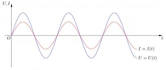
Recall that the instantaneous value of alternating current can be expressed as a harmonic oscillation
where - any point in time
- angular frequency
— initial phase
In the same way we can represent the instantaneous voltage values
If we try to estimate what the average current value will be over a certain period, we will encounter certain difficulties.
Since the instantaneous current over a period can take both positive and negative values, adding them up, we get that the average value of the current is zero. But this can’t be...
The current that passed during this period did some kind of work, but it could not disappear without anything, leaving no traces.
How much work can a current passing through a conductor do? The simplest and most noticeable process is heating the conductor. And according to the Joule-Lenz law, which determines how much electrical energy is converted into heat, there is a connection between heating (heat release) and the current value passing through the conductor.
Thus, experimentally, and then theoretically, it was determined that there is a simple relationship between the amplitude of the current and the “average” value (it is correct to call it effective ).
It is the effective value of the current that does the work and participates in power calculations. This is the value that the voltmeter shows when we measure AC voltage.
The same reasoning about tension leads us to a similar formula.
We can also represent harmonic oscillation in complex form (exponential form)
This is not our whim. This is just a desire to simplify the calculations that occur in electrical engineering.
For example, when adding two periodically changing current values, it is better to use vector addition. What is vector addition if not working with complex numbers? And so it is in everything in electrical engineering.
Therefore, we can express the value of the actual current like this
Then, knowing the complex values of current or voltage in the form , we can find out the absolute value of the current , as well as the initial phase
General electrical engineering (page 25)
In electrical circuits, non-sinusoidal current can be present in two cases:
· under the influence of sources of non-sinusoidal voltage or current;
· due to the nonlinearity of the elements of the electrical circuit.
1. Methods of representing non-sinusoidal functions
When calculating non-sinusoidal alternating current circuits, the expansion of periodic functions into one of the forms of the harmonic Fourier series is used. If a function with period T
is represented by the sum of
instantaneous values of harmonic oscillations
of various frequencies, where
k
= 1, 2, ¼ ordinal number of the harmonic, then the Fourier series is written in the following form
where is the constant component of the function, equal to its average over the period T
meaning;
and are the Fourier series coefficients corresponding to the amplitudes of the harmonics of the quadrature components;
– amplitude
of the kth
harmonic;
– initial phase
of the kth
harmonic.
Dependences on the serial number k
The th harmonic (or its frequency) is usually called the amplitude and phase spectra of the oscillation, respectively. For periodic non-sinusoidal oscillations, the amplitude and phase spectra are discrete in nature, and the distance along the frequency axis between adjacent spectral lines is equal to . Theoretically, the Fourier series contains an infinite number of terms, but in most practical cases this series converges quite quickly, and calculations can be limited to a relatively small number of harmonics.
2. Energy characteristics of non-sinusoidal current
When calculating the energy characteristics in non-sinusoidal periodic current circuits, the following quantities are used:
effective voltage values U
and current
I
;
average power P
;
reactive Q
and full
S
power, as well as
· distortion power D
, distortion and power factor ,;
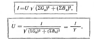
RMS voltage and current values
defined as the geometric sum of the effective values of individual harmonics
Where –
effective value
of the kth
voltage harmonic;
–
effective value
of the k
-th current harmonic;
–
constant components of voltage and current, respectively.
Average power
non-sinusoidal current is determined as the sum of the powers of individual harmonics
,
where is the average power k
th current harmonic;
– DC power.
Full power
non-sinusoidal current is determined similarly to the total power of a sinusoidal current using the formula
S = UI.
By analogy with sinusoidal current, the concept of reactive power
,
where is reactive power k
th current harmonic;
In contrast to sinusoidal current, the total power S
turns out to be greater than the geometric sum of average and reactive powers
3. Calculation of non-sinusoidal alternating current circuits
For non-harmonic influences, the circuit calculation algorithm can be as follows:
1) periodic non-harmonic influence is represented as a sum of harmonic signals
, using Fourier series;
2) limit the infinite Fourier series to a certain number of harmonics
, taking into account that the power of each subsequent harmonic decreases in proportion to the square of its amplitude;
3) perform a circuit calculation for each individual harmonic of voltage or current, taking into account that the structure of the circuit is preserved, and the resistance and conductivity of the reactive elements change
with a change in harmonic frequency;
4) the resulting response of the circuit is found using the superposition method by adding the reactions for individual harmonics of the influence.
In table 1. Some typical functions and their expansions in Fourier series are given. The graphs of these functions are shown in Fig. 4.1. The following designations are used: .
Table 4.1. Fourier series for non-sinusoidal functions Fig. 4.1. *
| Function graph no. | Fourier series expansion of a function |
| 1 | 2 |
| 1 | |
| 2 | |
| 3 | |
| 4 | |
| 5 | |
| 6 | |
| 7 | |
| 8 | |
| 9 | |
| 1 | 2 |
| 10 | |
| 11 | |
| 12 | |
| 13 | |
| 14 | |
| 15 | |
| 16 | |
| 17 | |
| 18 | |
| 19 | |
| 20 | |
| 21 | |
| 22 | |
| 23 | |
| 1 | 2 |
| 24 | |
| 25 | |
| 26 | |
| 27 | |
| 28 |
It should be remembered that for calculations these functions must be reduced to the form:
The conversion is carried out as follows:
TASK 4
Given:
A non-sinusoidal periodic voltage is applied to the electrical circuit, the diagram of which is given below, the shape of which is also shown. The circuit parameters have the following values: [Ohm]; [Gn]; [uF]; [IN]; [rad/s].
The following operations are required:
1) imagine the source voltage f
(
x
)=
e
( w
t
) by the Fourier series, limiting the number of terms of the series to the constant component and the first three harmonics.
2) construct graphs of the amplitude spectra and initial phases of a given source.
3) determine the load voltage using the complex value calculation method;
4) construct graphs of spectral components for voltage (current) at the load.
5) determine the effective value of voltage (current) at the load and the power dissipated in it.
| A ) Circuit diagram ( a ) and the shape of the input voltage ( |
Solution
1.
Let's use the data in table. 1 (function) and represent the source voltage in the form of a Fourier series limited by the constant component and the first three harmonics
2.
Let us plot the spectra of the amplitudes and initial phases of the source voltage, which are shown in Fig.
4.3 a
,
b
. When constructing graphs, we use a scale in which one division along the ordinate axis corresponds to 10 V, and along the abscissa axis – 100 Hz.
| A ) Rice. 4.3. Amplitude spectra ( a ) and phases ( |
3.
Now let's calculate the voltage on the load using the complex amplitude method.
For DC component
voltage across the load using the equivalent circuit shown in Fig.
4.4 a
, we get the following value
[IN].
When performing this calculation, it is taken into account that at a constant current the inductance must be replaced with jumpers, and the capacitance must be replaced with an open circuit, as shown in the figure below. The current in the load is determined by Ohm's law
[A].
When calculating the load voltage for harmonics EMF e
(
t
) source, you can use the equivalent circuit shown in Fig. 4.4
b.
In this diagram, all circuit elements are replaced by their complex resistances, which have double indices. The first index corresponds to the serial number of the branch, and the second – to the harmonic number. We determine the complex values of currents in the branches using the formulas
where is the equivalent complex resistance of the circuit for k
-th harmonic of the source voltage;
which take into account that the current is divided in the branches of the circuit into two currents, which are inversely proportional to the resistance of the branches.
| A ) ) and variable ( |
For the first harmonic,
using an equivalent circuit, we obtain the voltage across the load
[IN]; [Ohm]; [Ohm]; [Ohm] – circuit resistance for the first harmonic of the source voltage.
The complex amplitude of the first harmonic current of the source matters
[A]
This current is divided inversely proportional to the resistances of parallel-connected branches and, therefore the current in the load
[A]
We determine the complex value of the voltage at the load using Ohm’s law
[IN]
The resulting value allows you to record the instantaneous value of the first voltage harmonic at the load
[IN]
Second harmonic
Let's determine the load voltage using the equivalent circuit in Fig.
4.4 b
circuit resistance and source voltage for the second harmonic
[IN]; [Ohm]; [Ohm]; [Ohm].
The value of the complex amplitude of the second harmonic current in the voltage source circuit will be found using Ohm’s law
[A]
Complex amplitude of the second harmonic current in the load R
n we will find similarly to the first harmonic current by dividing the source current inversely proportional to the resistance of the parallel-connected branches
[A]
We find the complex value of the second harmonic voltage at the load using Ohm's law
[IN]
The resulting value allows you to record the instantaneous value of the second harmonic voltage at the load
[IN]
fourth harmonic voltage
Let's do it in the same way as calculating the second harmonic voltage. Circuit resistances and source voltages for the fourth harmonic have the following values:
IN; [Ohm]; [Ohm]; [Ohm].
We determine the complex amplitude of the fourth harmonic current using Ohm’s law
[A]
Using the fourth harmonic current in the branch with the voltage source, we calculate the current in the load
[A]
The complex value of the fourth harmonic of the voltage at the load is determined by Ohm’s law
[IN]
The instantaneous value of the second voltage harmonic at the load is determined by the formula
[IN]
We find the resulting load voltage by summing the individual components calculated above
Let's imagine the graphs of the emf of the source e
(
t
) and load voltage
4.
Let's plot the spectral components of the voltage across the load using the instantaneous voltage value obtained above. These graphs show that the electrical circuit connected between the source and the load has a certain smoothing effect: the amplitudes of the spectral components decrease as the frequency increases. In addition, a significant delay of the signal with respect to the source voltage is noticeable.
5.
Let us determine the effective voltage across the load and the average power dissipated in it. The effective voltage at the load can be calculated using the formula:
where =31.80 V is the constant component of the voltage across the load;
V – effective value of the first harmonic voltage;
V – effective value of the second harmonic voltage;
V is the effective value of the fourth harmonic voltage.
The average power of a non-sinusoidal current is determined by the formula:
where W is the power of the direct current component;
W – average power of the first harmonic current;
W – average power of the second harmonic current;
W – average power of the fourth harmonic current.
From the obtained expressions it follows that the average power is almost completely determined by the direct component and the first harmonic of the current. The contribution of higher harmonics is very insignificant and amounts to only 1.6% of the total power dissipated in the load.
TASK 4
For a given electrical circuit diagram, the structure of which is shown in Fig. 1 or 2 and parameters from tables 4.1...4.4, perform:
1) represent a given function of an EMF or current source in a Fourier series, limiting the number of terms of the series to the constant component and the first three harmonics.
2) construct graphs of the amplitude spectra and initial phases of a given source.
3) determine the function - voltage or current at the load, using the complex value calculation method;
4) construct graphs of spectral components for voltage (current) at the load.
5) determine the effective value of voltage (current) at the load and the power dissipated at the load.
Fig.1 Fig.2
Before the calculation in accordance with the task option, it is necessary to draw up an electrical diagram of the circuit, replacing the structural elements with elements
R ,
L
and
C. As an example, let's draw up a diagram of option 29 of table 4.1
| Due to the large volume, this material is placed on several pages: 25 |
Get text
Fundamentals of complex calculation of electrical circuits
Definition 1
Complex current is the complex effective value of a sinusoidal current.
One of the main ways to calculate AC electrical circuits is the symbolic or complex method. Typically, it is used in the analysis of electrical circuits with harmonic currents, voltages and electromotive force. As a result of the solution, a complex value of voltages and currents is obtained. A sinusoidal quantity can be represented:
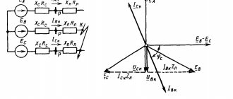
- In the form of a rotating vector.
- As a complex number.
An example of a rotating vector is shown in the figure below.
Figure 1. An example of a rotating vector. Author24 - online exchange of student work
Are you an expert in this subject area? We invite you to become the author of the Directory Working Conditions
From this figure it can be seen that the sinusoidal value a changes over time, which can be the input voltage or any other parameter of the electrical network. The quantity has a certain initial value (t=0) at the initial phase φ:
Figure 2. Formula. Author24 - online exchange of student work
At angle Wt3, when the sum Wt3+ф=90 and accordingly:
Figure 3. Formula. Author24 - online exchange of student work
Finished works on a similar topic
Course work Integrated calculation of electrical networks 480 ₽ Abstract Integrated calculation of electrical networks 220 ₽ Test work Integrated calculation of electrical networks 220 ₽
Receive completed work or specialist advice on your educational project Find out the cost
The sinusoidal value at angle Wt7, when the sum Wt7 + f = 270 will have a negative value:
Figure 4. Formula. Author24 - online exchange of student work
The value will have a negative value at angles Wtn + φ = 0, when Wtn = –φ (this area is not marked in the figure), thus:
Figure 5. Formula. Author24 - online exchange of student work
Also, the sinusoidal value will have a zero value at angle Wt11, when Wt11+ ph = 360:
Figure 6. Formula. Author24 - online exchange of student work
It is according to this law that a sinusoidal quantity, for example voltage, can change, changing from 0 to the maximum value and back.
Another form of presentation is complex
Figure 7. Formula. Author24 - online exchange of student work
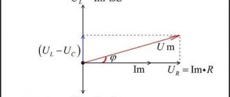
To do this, construct a graph (complex plane) of the dependence of two quantities, as in the figure below.
Figure 8. Graph. Author24 - online exchange of student work
The length of the vector Am is equal to the maximum value of the amplitude of the quantity under consideration. If we take into account the initial phase (φ), then this number is written as follows.
Figure 9. Formula. Author24 - online exchange of student work
In practical calculations of the complex method, it is not the amplitude value that is used, but the effective value, which is less than the root of 2 amplitude:
Figure 10. Formula. Author24 - online exchange of student work
When working with complex numbers, one of three ways to write a complex number is used: trigonometric form, algebraic form, exponential form. For example, there is a complex number in exponential form:
Figure 11. Formula. Author24 - online exchange of student work
In trigonometric form it will look like this:
Figure 12. Formula. Author24 - online exchange of student work
As a result, when moving to algebraic form, considering that:
Figure 13. Formula. Author24 - online exchange of student work
we get:
Figure 14. Formula. Author24 - online exchange of student work
where, ReA = 8.66 – real component of a complex number; ImA = 5 – imaginary component of a complex number.
When passing from the algebraic form to the exponential form, we obtain a number of the following form
Figure 15. Formula. Author24 - online exchange of student work
It goes to exponential form by the following transformation:
Figure 16. Formula. Author24 - online exchange of student work
And the angle is calculated by the formula
Figure 17. Formula. Author24 - online exchange of student work
And in the end it turns out:
Figure 18. Formula. Author24 - online exchange of student work
Effective value complex
Representation of sinusoidal currents and voltages using vectors on the complex plane. Complex amplitude.
Effective value complex
We have already depicted currents and voltages in the form of vectors, all that remains is to take the complex plane:
Unlike mathematics, the imaginary unit is denoted by the letter, because denotes the instantaneous current value.
The length of the complex vector is equal to the amplitude or effective value. In the first case, it is called complex amplitude
, in the second –
by the complex of the effective value
. The angle of rotation corresponds to the phase.
As is known from mathematics, complex numbers have two main forms of notation: algebraic and exponential. There is also a trigonometric form, but it is like a transition from exponential to algebraic, so no attention is paid to it.
is the complex amplitude in exponential notation.
This is not a prime complex number, it is a time function, so to distinguish it from prime complex numbers, which are denoted by an underscore, the complex amplitude is denoted by a dot at the top.
To obtain the complex effective value, you need to divide the complex amplitude by:
This is also a complex function of time, so it is indicated by the dot above.
Similar to currents, complex amplitudes and complexes of effective voltage values are introduced.
In order to move from complexes to instantaneous values, you need to take projections of the complex amplitude onto the imaginary axis:
The complex amplitude vector, as well as the complex effective value vector, rotates on the complex plane with an angular frequency (cyclic frequency). It is impossible to work with such vectors. To stop this vector, take time = 0: ; Then
The transition from the exponential form to the algebraic form is carried out through the trigonometric form. It is necessary to take projections of the complex vector onto the real axis – and onto the imaginary axis.
(Euler formula)
To move from algebraic to exponential form, use the following formula:
Attention!!! This formula works if the vector is in the 1st or 4th quarter of the complex plane, i.e. when, if (the vector is in the II or III quarter), then you need to use another formula:
those. multiplying a complex vector by is equivalent to rotating it on the complex plane by one time, and multiplying by –
equivalent to turning one time.
So,
Conclusions:
Sinusoidal periodic functions of currents and voltages can be associated with temporary functions on the complex plane, which are called images and carry all the information about the real functions (currents and voltages), their amplitudes and phases, therefore Kirchhoff’s laws are satisfied for complex functions. Addition, subtraction, division, multiplication, differentiation and integration of real functions can be replaced by the same operations with complex images.
| | | next lecture ==> | |
| triangles of voltage, resistance, power | | | Complex voltages (on resistances, inductances and capacitances). Complex resistances. Ohm's laws in complex form |
Date added: 2016-05-28; views: 6615; ORDER A WORK WRITING
Find out more:
Application of complex numbers in electrical engineering
The first mention of “imaginary” numbers as square roots of negative numbers dates back to the 16th century. The Italian scientist Girolamo Cardano (1501-1576) published a work in 1545 in which, trying to solve the equation
, he came to the expression
. The real roots of the equation were represented through this expression:
Thus, in Cardano's work, imaginary numbers appeared as intermediate terms in calculations. Cardano's merit was that he allowed the existence of a “non-existent” number
, introducing the multiplication rule: everything else became a matter of technique.
However, for another three centuries, mathematicians got used to these new “imaginary” numbers, from time to time trying to get rid of them. Only since the 19th century, after the publication of the works of Carl Friedrich Gauss (1777-1855), devoted to the proof of the fundamental theorem of algebra, complex numbers took root in science.
Complex numbers are one of the most suitable sections of the mathematical analysis course for the implementation of the professional orientation of bachelors in the field of preparation Informatics and Computer Science. When studying complex numbers, it is necessary to take into account the application of mathematical knowledge in general technical and special disciplines, in particular electrical engineering. The use of complex numbers makes it possible to use laws, formulas and calculation methods used in direct current circuits to calculate alternating current circuits, to simplify some calculations by replacing the graphical solution using vectors with an algebraic solution, to calculate complex circuits that cannot be solved in any other way, to simplify calculations DC and AC circuits.
When calculating circuits, it is necessary to carry out mathematical operations with complex numbers, so students must be able to perform the following operations: 1) find the modulus and argument of a complex number and a complex number by modulus and argument; 2) convert a complex number from one form to another; 3) perform addition and subtraction, multiplication and division of complex numbers.
In addition, it is very important to teach how to construct a curve and a vector from a sinusoid equation, a vector from a complex number, determine a complex number from a vector and an equation, an equation from a complex number.
In electrical engineering, the topic “Alternating current” occupies a significant place. This is explained by the fact that most electrical installations operate on alternating current, which varies sinusoidally.
The alternating voltage equation has the form , where u is the instantaneous voltage value;
–maximum value (amplitude) of voltage; w
– angular frequency
; t
– time
;
– initial phase angle
;
– electric angle
.
This equation relates two variables: voltage
u
and time
t
. Over time, the voltage changes sinusoidally.
The equations of other sinusoidally varying quantities have a similar form: current, emf.
etc.
When calculating AC circuits, it is necessary to use sinusoidally varying quantities, i.e. perform addition, subtraction, multiplication and division of equations of the above type.
Adding sinusoidal quantities is labor-intensive, especially if you have to add a large number of equations. A sinusoidal quantity is uniquely represented by a rotating vector, the length of which is equal to the amplitude, and the initial position is determined by the angle
, the vector rotates with angular velocity w
. Operations are performed with equations that have the same angular frequency, that is, all vectors that replace the equations rotate at the same angular speed. Consequently, their relative position does not change, and there is no need to rotate the vectors. Since vectors replace sinusoidal quantities, it is possible to replace addition or subtraction with addition or subtraction of vectors.
A variable sinusoidal value has the following properties:
1. A variable sinusoidal quantity can be uniquely represented by a vector. The length of the vector is equal to the amplitude; the tilt angle is equal to the initial phase angle.
2. Addition (and subtraction) of sinusoidal quantities can be replaced by addition (and subtraction) of vectors.
In addition to addition and subtraction, sinusoidal quantities must be multiplied and divided. This is where complex numbers come to the rescue.
A complex number can be represented on a plane by a vector whose length is equal to the modulus of the complex number, and the angle of inclination is equal to the argument. In electrical engineering, unlike mathematics, the imaginary unit is denoted by the letter j
.
If there is a complex number A = a + jb ,
then it can be represented as a vector, where
– modulus of a complex number;
is the argument of a complex number.
A complex number has three forms: algebraic – A = a + jb ;
trigonometric -
; indicative -
.
A complex number is uniquely represented by a vector, and a certain vector corresponds to a certain complex number.
Thus, if a variable sinusoidal quantity can be represented by a vector, and a certain vector corresponds to a certain complex number, then a variable sinusoidal quantity can be represented by a complex number.
Quantities such as voltage and current, resistance and conductivity, power are expressed in complex numbers.
Voltage and current.
There is an equation
.
In electrical engineering, the vector length is taken not to be the maximum, but the effective value. It is denoted by a capital U
without a subscript and is calculated by dividing the maximum value by
.
A sinusoidal quantity expressed as a complex number is called a complex
and is indicated by a capital letter with a dot at the top. The stress complex can be written in three forms: algebraic -, trigonometric -
and indicative -
.
Thus, in the voltage complex, the module is equal to the effective value, the argument is equal to the initial phase angle, the active component is equal to the real part of the voltage complex, and the reactive component is equal to the imaginary part.
Similarly for current: ,
, , ,
.
Example.
Given: current in complex form
Write the current equation.
Solution.
In order to write the equation, you need to know the amplitude and initial phase angle. Therefore, it is necessary to find the module - the effective value and the argument - the initial phase angle of the given current complex:
,
,
,
.
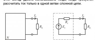
Resistance and conductivity.
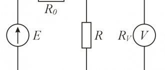
There is a circuit (Fig. 1):
r
– active resistance (incandescent lamp);
– inductive reactance (coil);
z
is the total resistance of the circuit, called total.
Fig.1 Fig.2
Resistances r , ,
z
form a right triangle of resistance (Fig. 2). Corner
– phase shift angle.
Resistances are not sinusoidal quantities, but the segment z
can be expressed as a complex number, considering that the segment
r
is plotted along the axis of real numbers, and the segment along the axis of imaginary numbers.
Resistance in complex form is denoted by the letter Z
. For the circuit in Fig. 2, the resistance complex is written:
– algebraic form;
– trigonometric form; - demonstrative form.
Module ; argument
. Thus, in the resistance complex, the modulus is equal to the total resistance, and the argument is equal to the phase shift.
Power.
The power complex is obtained if the voltage complex is multiplied by the conjugate current complex: , where
– power complex, – conjugate current complex.
After multiplication, we obtain a complex number whose real part is equal to the active power, and the imaginary part is equal to the reactive power:
, where P is active power, Q is reactive power.
Example.
,6; . Determine active P and reactive power Q.
Solution.
Let's translate the voltage and current complexes into exponential form; to do this, we find the modulus and argument of the current and voltage:
, ,
,
, , .
Let us define the conjugate current complex:
,
Let's find the active and reactive power: P=975W, Q=171 var.
The algebraic form of a complex number is convenient for addition and subtraction, and the exponential form for multiplication and division; trigonometric is used to convert exponential form into algebraic form.
In classes, teachers can use examples without going in depth into electrical engineering, considering tasks only from a mathematical point of view. As additional material and independent work, you can offer tasks like:
- Given: a) ; b)
; V)
; G)
Find the modulus and argument of a complex number.
- Given: a)
; b); V)
.
Write complex numbers in exponential and algebraic forms.
- Given: a)
; b) ; V)
;G) ; d)
; e)
; and)
.
Convert the algebraic form of a complex number to the exponential form and vice versa.
- Perform addition, multiplication, division of complex numbers.
Given: a) ; b)
; V)
.
This article will help mathematics teachers understand the issue of the application of complex numbers in electrical calculations.
Literature:
- Theoretical foundations of electrical engineering: Theory of electrical circuits and electromagnetic fields: textbook. aid for students higher textbook institutions / ed. S.A. Basharina, V.V. Fedorov. – M.: Publishing House, 2004. – 304 p.