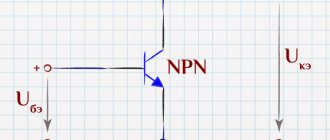
What is an amplifier?
Low power signals are very common in electrical circuits. For example, this could be an audio signal from a dynamic microphone
weak radio signal that your Chinese radio picks up from the air
Or a reflected signal from an enemy missile, which is then caught, amplified and tracked by a radar installation. For example: TOP anti-aircraft missile system:
As you can see, in electronics absolutely everywhere there is a need to amplify weak signals. In order to amplify them, you need signal amplifiers. Amplifiers are widely used in radar, television, radio broadcasting, telemetry, computer technology, automatic control, automation systems, etc.
What is a black box in electronics
In general, an amplifier can be viewed as a black box.
What is this black box? This is a box. He's black). And since it is black, absolutely no one knows what is in it. We can only guess. But it is also possible that we can take some action and wait for a response. After the response of this black box, we can guess what is inside it.
That is, in essence, a black box must have some “sensors” for perceiving information from the outside, some “input”, as well as some “output” for a response. That is, by applying any influence to the input, we wait for the response of the black box at the output.
Let there be a cat or cat in the black box, but so far no one knows that he/she is there. What will we do first? Let's shake the box or kick it, right? If someone meows there, it means it’s definitely either a cat or a male cat). That is, there was a response. How to determine further whether it is a cat or a male cat? We open the box, and a shaggy miracle crawls out of it. If it runs, it means it's a cat. If it runs, it means it’s a cat).
But there can also be absolutely any body or substance in the black box. For such situations, we must conduct as many experiments as possible, that is, produce as many input influences as possible to more accurately determine the contents of the black box.
Differentiator
The differentiator's action is opposite to that of the integrator, that is, the output signal is proportional to the rate of change of the input signal. The simplest differentiator diagram is shown below
Differentiator on an operational amplifier.
The differentiator implements the differentiation operation on the input signal and is similar to the action of differentiating RC and RL chains, in addition, it has better parameters compared to RC and RL chains: it practically does not attenuate the input signal and has a significantly lower output resistance. The basic calculation relationships and response to various impulses are similar to differentiating chains.
The output voltage will be
What is a quadripole
In electronics, a black box is a quadripole . What is a quadripole anyway? A four-terminal network is a black box containing an unknown electrical circuit inside. Here we see two input terminals, through which the input action is supplied, and two output terminals, from which we will now take the response of our “electric black box”.
Passive quadripole
For example, an RC circuit is a passive four-terminal network , since it has four terminals: two for input and two for output, and as we can see, it does not contain any power supply. This RC circuit is a passive low pass filter (LPF).
In passive two-terminal networks, the voltage or current at the output can be greater than at the input, but the power does not increase. How can the voltage or current at the output be greater than at the input? Here it is enough to recall the transformer, as well as series and parallel oscillatory circuits. For them, it would be more accurate to define a voltage converter, but not an amplifier, since the amplifier must include a power source from which it will take energy to amplify a weak input signal.
Also, in a passive four-port network, the output power will in no way be greater than the input power. If you achieve this, you will immediately receive an eternal source of energy and a Nobel Prize to boot. But remember that the law of conservation of energy, which was first formulated by Leibniz in the 17th century, has not been canceled.
Active quadripole
But we will now call this four-terminal network active , since it includes a power supply +Upit, which is required in order to amplify the signal.
That is, here we see two terminals for the input, to which the signal Uin is driven, and we also see two terminals for the output, where the voltage Uout is removed. Our four-port network is powered via + Upit, as a result of which, in this case, the output signal will be greater than the input signal.
By driving a sinusoid into the input of such a circuit, at the output we will get the same sinusoid , but its amplitude will be many times greater.
This is, of course, true for an ideal amplifier, i.e. absolutely linear and without restrictions on the amplitude of the input and output signals. In real amplifiers, it is required that the amplitude does not exceed the permissible value and that the amplifier is properly designed. In addition, any real amplifier introduces distortion and is characterized by nonlinear distortion coefficient (THD) and many other parameters, which we will consider in the next article.
In an active four-port network , one of which is a power amplifier, the output power will be greater than the input. Naturally, this does not violate the law of conservation of energy, since the power released to the load is the converted power of the power source. The small signal input simply controls this power. You can read more in the article about the principle of transistor amplification.
In electronics, we will consider an amplifier as an active four-port network , to the input of which a low-power signal Uin is supplied, and a load Rн is attached to the output.
Integrator
The integrator allows you to implement a circuit in which the change in output voltage is proportional to the input signal. The circuit of the simplest op-amp integrator is shown below
Operational amplifier integrator.
This circuit implements the integration operation over the input signal. I have already looked at schemes for integrating various signals using integrating RC and RL chains. The integrator implements a similar change in the input signal, but it has a number of advantages compared to integrating chains. Firstly, RC and RL circuits significantly attenuate the input signal, and secondly, they have high output impedance.
Thus, the main calculated relations of the integrator are similar to the integrating RC and RL chains, and the output voltage will be
Integrators have found wide application in many analog devices, such as active filters and automatic control systems
Generalized amplifier circuit
It looks something like this:
As we can see in the diagram, some source of a weak signal with EMF EI and internal resistance RI is connected to the input of the amplifier stage through terminals 1 and 2. It is this weak signal from this source that we will amplify. Further, as expected, each amplifier has its own input resistance Rin. The current strength Iin in the circuit EI -> RI -> Rin, as difficult as it may be to guess, will depend on the input resistance of the amplifier stage Rin.
As you already know, the power supply plays a major role in the amplifier stage. A low-power, weak signal controls the energy consumption of the power supply. As a result, at the output we get an amplified copy of the weak input signal. The amplification occurred due to the fact that the power supply provided its power to amplify the input signal. Well, something like this).
In the output circuit of the amplifier we receive an amplified signal with EMF (What is EMF) Eout and output resistance Rout. Through terminal blocks 3 and 4 we connect the load Rн, which will already consume the energy of the amplified signal. The current strength in the circuit Eout -> Rout -> Rн will depend on the load resistance Rн.
Ideal operational amplifier and its properties
Since our world is not ideal, ideal operational amplifiers do not exist. However, the parameters of modern op-amps are at a fairly high level, so analysis of circuits with ideal op-amps gives results very close to real amplifiers.
To understand the operation of op-amp circuits, a number of assumptions are introduced that reduce real op-amps to ideal amplifiers. There are only five such assumptions:
- The current flowing through the op-amp inputs is assumed to be zero.
- The gain of the op-amp is assumed to be infinitely large, that is, the output voltage of the amplifier can reach any value, but in reality it is limited by the supply voltage.
- The voltage difference between the inputs of an ideal op-amp is zero, that is, if one of the terminals is connected to ground, then the second terminal has the same potential. It also follows that the input impedance of an ideal amplifier is infinite.
- The output impedance of an ideal op-amp is zero.
- The amplitude-frequency response of an ideal op-amp is flat, that is, the gain does not depend on the frequency of the input signal.
The closeness of the parameters of a real operational amplifier to the ideal ones determines the accuracy with which a given op-amp can operate, as well as find out the value of a particular operational amplifier and quickly and correctly select a suitable op-amp.
Based on the assumptions described above, it becomes possible to analyze and derive relationships for the basic circuits of the operational amplifier.
Amplifier types
Amplifiers can be divided into three groups:
Voltage amplifier
A voltage amplifier (VA) amplifies the input voltage a specified number of times. This coefficient is called voltage gain and is calculated by the formula:
Where
KU is the voltage gain
Uout - amplifier output voltage, V
Uin - voltage at the amplifier input, V
The output amplified voltage should not change from the load current, and therefore from the load resistance. Ideally, the output resistance Rout should be zero, which is unattainable in practice. Therefore, they try to design NAs in such a way as to minimize the output resistance Rout.
In this mode, the amplifier operates if the conditions are met that Rin is much greater than Rout, i.e. Rin >>Ri and Rn are much greater than Rout (Rn >>Rout). The higher the rating Rн, the better for the voltage amplifier, since the load will not sag the output voltage Uout. Everything is simple here: the lower the load resistance, the greater the current will flow through the circuit Eout -> Rout -> Rn, the greater the voltage drop across the output resistance Rout, based on the EMF formula: Eout = IoutRout + IoutRn. You can read about this in more detail in the article Ohm's Law for a complete circuit.
Current amplifier
The current amplifier (CA) amplifies the input current by a specified number of times. This coefficient is called the current gain and is calculated by the formula:
where KI is the current gain
Iout - current strength in the load circuit, A
Iin - current strength in the input circuit Ei ->Ri ->Rin, A
The meaning of the operation of the current amplifier is this: at a certain current strength in the input circuit, at the output in the load circuit we obtain a current strength that is KI times greater, regardless of what value the load rating takes. Ohm's simple law I=U/R already works here.
If the current strength must be constant, and our resistance value can be floating, then to maintain a constant current strength in the load circuit, our amplifier automatically changes the voltage Uout at the load. As a result, the current remained constant and remained the same. Or in letters: Rн =var, Iout= const.
You will tell your electronics teacher the above explanation, and now the explanation is for complete dummies . So, in the input circuit Ei -> Ri -> Rin, let us have a current flow of 10 mA. Coefficient KI = 100, therefore, at the output in the load circuit Eout -> Rout -> Rн a current with a force of 1 A (10 mA x 100) will flow. But such a current by itself will not flow through this circuit. It needs to create conditions for it to occur. Let's say we have a load of 10 ohms. What then should be the voltage in this circuit to obtain a current in this circuit of 1 A? Remember Uncle Om: I=U/R. 1=Uout/10, we get U=10 V. This is the voltage the current amplifier will give us at the output.
But what if the load changes its value? The current should remain the same, do not forget, that is, 1 A, since this is a current amplifier. In this case, so that the current in the circuit remains 1 A, the amplifier will automatically change its voltage value at the output Uout to 1=Uout /5. Uout =5/1=5 V. That is, we will already have 5 Volts at the output.
But we also do not forget about one more parameter, which is located in the output circuit of the current amplifier. This is the output resistance Rout. Therefore, we need the following condition to be satisfied: Rin << Ri and Rn << Rout at which the specified current in the load is ensured at a low voltage value.
Amplifier
It used to be very cool and fashionable to assemble power amplifiers (PA) with your own hands, turn on Tender May and turn the volume up to full blast. Now everyone can assemble or buy UM, since the Internet and Aliexpress are always at hand.
How does UM differ from UN and UT?
If in the UT we increased only the current, in the UN we increased the voltage, then in the UM we increased the current and voltage by a multiple of times.
The power formula for direct and alternating current with a resistive load looks like this:
Where
P—power, W
I - current strength, A
U—voltage, V
Therefore, the power gain will be written as:
Where
KP - power gain
Pout - amplifier output power, W
Pin - power at the amplifier input, W
For a power amplifier, the conditions for matching the input circuit with the source of the input signal and the output circuit with the load for transmitting maximum power have the form: Rin ≈ Ri and Rn ≈ Rout.
Also, do not forget that loads can be either purely active (such as an incandescent light bulb, a resistor, various heaters) or have a reactive component (inductors, capacitors, motors, etc.).
General information about electronic amplifiers
2.1.1 Electronic amplifier structure
An electronic amplifier is a device that converts a low-power input electrical signal into a signal of much higher power with minimal distortion of its shape. Signal power can be amplified by current or voltage amplification.
The amplification effect is only possible if there is an additional source of energy, called a power supply. Therefore, an amplifier is a device that, under the influence of an input signal, converts the energy of a power source into the energy of an output (useful) signal.
A generalized circuit diagram for switching on the amplifier is shown in Figure 2.1.
Figure 2.1 – Circuit diagram for connecting an electronic amplifier
The source of the input signal of the amplifier can be any converter of an electrical or non-electrical quantity into an electrical one: a microphone, a photocell, a piezoelectric element, a magnetic readout head, a previous amplifier, a thermoelectric sensor, a chemical current source, etc. Depending on the type of source, the power range of the signals received to the amplifier input, wide enough. For example, the voltage supplied to the amplifier input from the transmitting television tube is only 2 ... 5 mV at low power. A voltage not exceeding tenths - hundredths of a millivolt can be supplied from the microphone to the input of the amplifier. However, sources such as the preceding amplifier can create voltages reaching tens to hundreds of volts with a signal power of a few watts.
The amplifier's electrical output goes to a device called a load. Various converters of electrical energy into electrical or non-electrical energy can be used as an electronic amplifier load: telephone, loudspeaker, galvanometer, relay, subsequent amplifier, electric motor, lighting or heating devices, etc. The power consumption values for various types of load lie within wide limits. For example, the power consumed by a telephone is hundredths of a watt. At the same time, the power consumed by the city's wired broadcasting network reaches hundreds of kilowatts.
The electronic amplifier can be single-stage, two-stage or multi-stage. In general, an amplifier consists of several stages, the first of which is connected to the signal source, and the load to the output of the last. The need to use several cascades is due, first of all, to the fact that the signal transmitted from the source to the load must first be amplified by thousands - tens of thousands or more times. When used in an amplifier as an active element, for example, a bipolar transistor with a base current transfer coefficient of 50 ... 100, the problem can only be solved if several amplification stages are connected in series. In addition, it often becomes necessary to match the output impedance of the signal source with the input impedance of the amplifier, or the output impedance of the amplifier with the load impedance.
A generalized block diagram of an electronic amplifier is shown in Figure 2.2.
The amplifier includes the following elements:
— final amplifier stage (OK), designed to amplify the signal power and allocate it to the load (N);
— pre-terminal stage (POC), designed to control transistors of the final stage. When the power of the final stage is high, the SOC must provide power sufficient to obtain the required undistorted output power of the amplifier. If the final stage is push-pull, then the pre-final stage simultaneously inverts the phase of the signal voltage;
— pre-amplification stages (PrA) (their number is determined taking into account the required voltage amplification factor), which serve to increase the level of signals received from the source (IC) to the value necessary to control the transistors of the pre-final stage;
— an output device (Output), which serves to match the load resistance with the output resistance of the final stage, balance the output circuit, and also to isolate the load circuit from constant voltages and currents acting in the amplifier circuits;
— an input device (IDU), which serves to match the internal resistance of the signal source with the input resistance of the first stage of the amplifier, to balance the input circuit of the amplifier, and also to isolate the signal source circuit from constant voltages and currents acting in the input circuits of the amplifier;
- a general negative feedback circuit (GNF), which serves to reduce distortion and noise, stabilize gain, and also to stabilize the initial modes of transistors (for these purposes, separate AC and DC NFB circuits can be used). The NFB circuits may or may not cover the output device, and may also cover all or part of the preamp stages;
— inertia-free protection device (UBZ) – to protect the transistors of the final stage of the amplifier from overload;
— power supply and filters (FP) in the power circuits of the pre-amplifier stages.
Figure 2.2 – Generalized block diagram of the amplifier
However, in each particular case, the amplifier block diagram may not contain all the elements shown in Figure 2.2. Thus, in the case of using a single-ended final stage of low power, the pre-final stage does not differ from a conventional pre-amplifier stage and therefore should not be considered as a special element of the structural circuit. In addition, there may be no instantaneous protection devices or other elements shown in Figure 2.2.
2.1.2 Classification of amplifiers
Electronic amplifiers are used in a wide variety of fields of science, technology and production. Being either independent devices or part of more complex devices and systems, amplifiers have found wide application in radio broadcasting, sound cinema, sound recording technology, television, radar and radio navigation, nuclear physics, medicine and biology, computer technology, automation systems, measuring technology and etc. Despite such a wide range of application areas, amplifiers designed for completely different purposes can have identical properties. Therefore, the classification of amplifiers by purpose, as a rule, is not used, since it provides little information for judging the properties and features of such devices.
Typically, when classifying amplifiers, the following are taken into account:
— character (shape) of the input signal;
— range of amplified frequencies;
- functional purpose;
- type of reinforcing elements.
Based on the shape of the amplified signals, continuous amplifiers and pulsed signal amplifiers are distinguished. The first include amplifiers of quasi-harmonic signals, for example speech, music, which change relatively slowly over time, so that transient processes in the amplifier almost do not appear. The properties of such amplifiers are assessed by the quality of harmonic vibration transmission. Pulse signal amplifiers are designed to amplify pulses, such as radar, television, telegraph, etc. This is where transient processes occur. Therefore, the properties of such amplifiers are assessed by the shape of the transient response.
Based on the frequency range, amplifiers are divided into direct current amplifiers (DCA) and AC amplifiers . DC amplifiers are those amplifiers that amplify oscillations with frequencies starting from fn = 0 to a certain (usually not very high) frequency fv, that is, they are capable of amplifying both the alternating and direct components of the input signal (Figure 2.3, a. Letter K Figure 2.3 indicates the gain of the amplifier). Amplifiers that can amplify only the AC component are called AC amplifiers. They amplify oscillations in the frequency range from the lower limit frequency fн to the upper limit frequency fв. Outside this frequency range, the width of which is called the passband, the gain drops below the permissible level (Figure 2.3, b, c).
AC amplifiers include:
- audio frequency amplifiers, the operating range of which is within 20 Hz ... 20 kHz, and fн << fв (Figure 2.3, b);
- radio frequency amplifiers, in which the ratio fв / fн is close to unity, and the frequency range is much higher than audio (Figure 2.3, c). These amplifiers are widely used in radio receiving devices. The output circuits of the cascades here include oscillatory circuits, the resonant frequency of which is fp "(fн + fв) / 2. Therefore, they are also called resonant amplifiers. Their bandwidth is Df = fв – fн<< fр. Other amplifiers, in contrast to resonant ones, are sometimes called aperiodic;
— broadband amplifiers (BA), in which fв > 100 kHz, and fн – tens of hertz. These include video path amplifiers in television equipment, video amplifiers for radar receivers, etc.
Figure 2.3 – Position of the passband on the frequency axis
for different classes of amplifiers
According to their functional purpose, amplifiers are conventionally divided into voltage amplifiers , current amplifiers and power amplifiers . This division is largely arbitrary. As noted earlier, power amplification can be achieved by voltage amplification, current amplification, or both voltage and current amplification. However, it is generally accepted that if the main purpose of the amplifier is to increase the voltage to the required level, then it is called a voltage amplifier. Current amplifiers are determined similarly. Power amplifiers are usually called the output stages of a multistage amplifier, capable of delivering the required power to an external load.
Based on the type of amplification elements, there are transistor , tube , dielectric , magnetic amplifiers and integrated circuit amplifiers .
In addition to the main classification characteristics considered, others can be used, for example: by type of power supply (battery, mains, etc.), by the number of cascades, by design (portable, stationary), etc.
2.1.3 Basic parameters and characteristics of amplifiers
The sum of information characterizing the basic properties of a technical device is called its indicators. Technical indicators of an electronic device characterize gain, distortion, conversion accuracy, input and output signal levels, etc. and allow one to assess the degree of suitability of the device for a particular application.
Let's consider the main technical indicators of electronic amplifiers. They can be divided into two separate groups - parameters and characteristics.
The main parameters of the amplifier include: input and output resistance, gain, permissible level of linear and nonlinear distortion, noise level, efficiency, dynamic range of the input signal.
Let's consider the listed parameters in more detail.
2.1.3.1 Input and output resistance. Input and output impedances are the most important parameters of amplification devices. Their values must be taken into account when matching the amplification device with both the input signal source and the load. In general, the values of the input and output resistances are complex and are a function of frequency .
The amplifier can be represented by an equivalent circuit shown in Figure 2.4. As can be seen from the figure, such a circuit is a four-terminal circuit - that is, an electrical system with four external terminals.
Figure 2.4 – Representation of an amplifier in the form of a four-terminal network
The input impedance of an amplifier is the internal resistance between its input terminals. In most cases, it is determined by the parallel connection of resistive (active) resistance Rin and capacitance Cw. The input impedance of an amplifier can be represented as the ratio of the complex amplitudes of the voltage between the input terminals of the amplifier and the current flowing in its input circuit:
. (2.1)
The value of the input resistance is selected either depending on the nature of the resistance of the signal source, or depending on the type of matching of the amplifier device with the signal source - current, voltage or power. It is usually desirable to provide a high resistance Rin and a low capacitance Cw. Some instrumentation amplifiers sometimes require that Rin ® 0.
The values of the voltage, current and power gains depend on the relationship between and . If you need to obtain the maximum voltage gain, then the condition must be met. To obtain the maximum current gain, it is necessary that , and for maximum power amplification, the equality must be fulfilled.
The output impedance of an amplifier is the internal resistance between its output terminals. In relation to the load, the amplifier is a source of a signal whose internal resistance is equal to
, (2.2)
where is the complex amplitude of the output voltage in idle mode (at RН ® ¥);
– complex amplitude of the output current during a short circuit in the load (RN = 0).
When choosing the value of the output impedance of the amplifier in each specific case, as well as when choosing the input impedance, they are approached individually. In general, you can use the same recommendations as when choosing an input impedance, namely:
- if you need to get the maximum voltage gain, then you must fulfill the condition
;
— to obtain the maximum current gain it is necessary that
;
— for maximum power amplification you need to fulfill the equality
.
2.1.3.2 Gain. Gain is one of the most important parameters of an amplifier. Depending on the type of amplified value, the amplification coefficients of voltage KU, current KI and power KP are distinguished.
voltage gain (voltage transfer) of an amplifier is the ratio of the amplitude or effective values of the output and input voltages:
. (2.3)
The gain is determined in steady state with a harmonic (sinusoidal) input signal.
The current amplification factor is the ratio of the amplitude or effective values of the output and input currents:
. (2.4)
The ratio of the power of the amplified oscillation in the load to the power of the signal supplied to the input of the amplifier is called power gain :
. (2.5)
When several amplification stages are connected in series, the overall gain of the system is determined as the product of the gains of the individual stages:
. (2.6)
In practice, gain factors are often expressed in logarithmic units - decibels. The power gain can be represented as follows
. (2.7)
If the powers RNi Rin are allocated at the same resistances (RN = Rin = R), then their ratio in decibels can be expressed through the voltage ratio
. (2.8)
Similarly, we can write for the current amplification factor
. (2.9)
Logarithmic units are convenient because they allow the multiplication of gain factors to be replaced by addition, that is
. (2.10)
If there are reactive elements in the amplifier stages (inductances, separating and blocking capacitors, capacitances of pn junctions of transistors, etc.), the gain should be considered as a complex quantity depending on the frequency
, (2.11)
where K(w) is the module of the complex gain;
j(w) is the argument of the complex gain, which is the phase difference between the output and input signals.
2.1.3.3 Linear distortion. Let us assume that the gain K(w) does not depend on the amplitude of the input signal. In this case, when a sinusoidal signal is applied to the input of the amplifier, the output signal will also have a sinusoidal shape, but will differ from the input in amplitude by K times and in phase by angle j.
According to Fourier's theorem, a periodic signal of complex shape can be represented as the sum of an infinitely large number of harmonic components having different amplitudes, frequencies and phases. Since K is a complex quantity, the amplitudes and phases of the harmonic components of the input signal when passing through the amplifier will change differently and the output signal will differ in shape from the input. Distortion of a signal when passing through an amplifier, caused by the dependence of the amplifier parameters on frequency and independent of the amplitude of the input signal, is called linear distortion .
In turn, linear distortions can be divided into frequency (characterizing the change in the magnitude of the gain K in the frequency band due to the influence of reactive elements in the circuit) and phase (characterizing the dependence of the phase shift between the output and input signals on frequency due to the influence of reactive elements).
Frequency distortions of a signal can be assessed using the amplitude-frequency characteristic, and phase distortions - using the phase-frequency characteristic.
2.1.3.4 Nonlinear distortions. As is known from the theoretical foundations of electrical engineering, if an electrical circuit contains at least one nonlinear element, then such a circuit is called nonlinear. Amplifiers include elements (devices) that have nonlinear current-voltage characteristics - transistors, diodes, magnetic circuits, semiconductor capacitors of microcircuits, etc. Therefore, if the operation of these devices is not ensured within the linear sections of the current-voltage characteristic, the gain of the amplifier will depend on the amplitude of the input signal, which, in turn, will cause nonlinear distortion of the amplified signal.
Thus, nonlinear distortions are understood as changes in the shape of the amplified oscillation caused by the dependence of the amplifier gain on the amplitude of the input signal.
When a signal passes through a nonlinear device (amplifier), its spectral composition changes - higher harmonics appear in its spectrum. A distinctive feature of nonlinear distortions is that even harmonic (sinusoidal) oscillations are subject to them. Nonlinear signal distortion in amplifiers is usually assessed using harmonic distortion.
The harmonic coefficient is the ratio of the effective value of the sum of the higher harmonics of the output voltage to the effective value of its first harmonic:
. (2.12)
The result will not change if in this formula we substitute not the effective, but the amplitude values of the harmonics, and instead of voltages we can operate with currents or powers
. (2.13)
Linear and nonlinear distortions characterize the accuracy of the amplifier's reproduction of the input signal shape.
Amplifiers with different purposes have different requirements for the value of harmonic distortion, which is usually expressed as a percentage. So, for example, for broadcast equipment with high quality speech and music reproduction it should not exceed 1 ... 2%, for devices of average quality - 5 ... 7%. Hi-Fi audio amplifiers usually provide Kg = 0.3 ... 0.5%. As practice shows, if the harmonic distortion does not exceed 0.2 ... 0.5%, then nonlinear distortions are practically invisible to the ear.
2.1.3.5 Efficiency. The efficiency factor (efficiency) h of the amplifier characterizes the efficiency of energy consumption of the power source. It is usually measured at a harmonic amplification frequency of 1 kHz. The overall efficiency of the entire amplifier is called industrial efficiency. It is the ratio of the rated output power supplied to the load to the total power consumed by the amplifier from all power sources:
. (2.14)
The difference РS – РН = Рpot is the power loss in the amplifier.
The higher the efficiency of the amplifier, the lower the power loss in it, which turns into heat. For example, to prevent overheating of the final transistors, they must be equipped with radiators, the dimensions of which can be smaller, the higher the efficiency. Thus, the efficiency of an amplifier also indirectly characterizes its specific dimensions and weight (per unit of output power).
2.1.3.6 Self-interference. The amplifier transmits to the output not only the amplified useful signal supplied to its input, but also unwanted oscillations that arise within it and are therefore called self-interference. The main ones are background, interference and noise, and in DC amplifiers - also zero drift.
Background is an oscillation with the mains frequency or a multiple of it. Usually it enters the amplifier through the power supply circuits due to insufficient smoothing of the ripples of the voltage source rectifier (when powered from an AC network). In tube amplifiers, an additional source of hum is the cathode filament circuits, if they are powered by alternating current.
Noise is called interference induced on the amplifier circuit by electric and magnetic fields. The sources of this interference may be the power supply's mains transformer, its connecting wires, power supply wires, or any electrical installations.
To quantify background and interference, use the ratio of their voltage at the output of the amplifier to the output harmonic voltage corresponding to the rated output power. For high-quality amplifiers, the background voltage should not exceed - 60 ... - 70 dB.
own noise is a fluctuation oscillation caused by the chaotic movement of free charge carriers (electrons and holes) in all electrically conductive materials from which the amplifier parts are made.
Noises arise at the microscopic level of the structure of materials and are therefore very weak. But, being amplified by a multistage amplifier, they can be commensurate with the level of the useful signal. Unlike background and interference, it is fundamentally impossible to completely eliminate the amplifier's own noise.
Zero drift is a slow change in the amplifier's output voltage due to instability of the supply voltage and transistor characteristics. Drift mainly occurs in DC amplifiers. It is quantified by the drift voltage or current converted to the input. The background level is sometimes assessed in the same way.
2.1.3.7 Amplitude and phase-frequency characteristics. As shown earlier, in general the gain of an amplifier is a complex quantity. Therefore, for the voltage gain we can write:
. (2.15)
As can be seen from the above formula, the modulus and argument of the complex voltage gain of the amplifier are functions of frequency.
The dependence of the modulus of the complex voltage gain of an amplifier on frequency (K(w)) is called the amplitude-frequency response (AFC) of the amplifier. A typical frequency response of an audio amplifier is shown in Figure 2.5.
Figure 2.5 – Typical amplitude-frequency response of an amplifier
For the frequency response of an amplifier, the presence of a so-called mid-frequency region is typical, within which KU is almost independent of frequency and takes its maximum value KU0. This is sometimes called nominal gain.
In the region of lower and upper frequencies, the frequency response usually decreases (the voltage gain decreases). The frequencies at which the module of the complex voltage gain decreases relative to its maximum value by a factor (in Figure 2.5 this level is shown as 0.707KU0) are called the cutoff frequencies of the amplifier (or frequency response cutoff frequencies): fн (wн) and fв (wв) - respectively lower and upper limit frequencies. The frequency range from wн to wв is called the amplifier bandwidth: .
Based on the amplifier's frequency response, frequency distortion can be determined in any operating frequency range. The characteristic of frequency distortion is the frequency distortion coefficient , determined from the ratio
, (2.16)
where KUf is the voltage gain at a given frequency.
Since the greatest frequency distortions occur at the boundaries of the passband, when calculating an amplifier, as a rule, frequency distortion coefficients are specified at the lowest and highest boundary frequencies. Usually they take Mn = Mv=, that is, at the boundary frequencies the voltage gain decreases to a level of 0.707 of the gain value at the middle frequency. Under such conditions, the bandwidth of audio amplifiers designed for reproducing speech and music lies in the range of 30 ... 20,000 Hz. For amplifiers used in telephony, a narrower bandwidth of 300 ... 3400 Hz is acceptable. To amplify pulsed signals, it is necessary to use broadband amplifiers, the bandwidth of which occupies a frequency range from a few hertz to tens or even hundreds of megahertz.
The dependence of the argument of the complex voltage gain of the amplifier on the frequency j(w) is called its phase-frequency characteristic (PFC). A typical phase response of an amplifier stage is shown in Figure 2.6 with a solid line.
The phase-frequency characteristic shows how the phase shift angle between the output and input signals changes when the frequency changes and determines phase distortion. There are no phase distortions if the phase-frequency characteristic is linear (dash-dotted line in Figure 2.6), since in this case each harmonic component of the input signal, when passing through the amplifier, is shifted in time by the same interval Dt. The phase shift angle between the input and output signals is proportional to the frequency
. (2.17)
Figure 2.6 – Phase frequency response of the amplifier
From Figure 2.6 it can be seen that within the amplifier’s passband, phase distortion is minimal, but increases sharply in the region of boundary frequencies. In particular, in an audio amplifier at the boundary frequencies, the phase shift angle between the input and output signals compared to this parameter in the middle of the passband is .
In a multistage amplifier, the frequency distortion coefficient is determined as the product of the corresponding coefficients of all stages
, (2.18)
and the phase shift between the output and input voltages is the algebraic sum of the phase shifts created by the individual stages
. (2.19)
2.1.3.8 Transient response. The transient response (TC) is the dependence of the instantaneous value of the output voltage uout(t) of the amplifier on time when a stepwise voltage drop uin(t) is applied to its input. The transient response determines the process of transition of the amplifier from one stationary state to another, when the input influence has abruptly changed by a certain value, conventionally taken as unity.
The transient response h(t), similar to the frequency response, is usually plotted on a relative scale (Figure 2.7), plotting vertically the ratio of the output voltage at each time t to its value in steady state: h(t) = uout(t)/Uout 0. At In practice, PHs are mainly used to evaluate the distortion of pulsed signals as they pass through an amplifier.
Distortion of intermittent (pulse) voltage is divided into two types: distortion associated with the increase in voltage, and distortion of its peak. The former are assessed by the rise (establishment) time tnar and the surge d, the latter – by the decline of peak D or its instability. The rise time is the time during which the front of the normalized PH increases from the level of 0.1 to the level of 0.9.
Figure 2.7 – Transient response of the amplifier
A surge is the maximum excess of the instantaneous voltage value over the steady-state value. The surge is expressed as a percentage of the steady-state voltage value. With the oscillatory nature of the process, there may be several noticeable spikes in the transient response. The largest of them is usually assessed.
The drop in the upper part of the normalized PC is also measured as a percentage of the steady-state value of the output voltage. It can be positive and negative (rise).
In amplifiers for high-quality reproduction of pulsed signals, the surge d and roll-off D should usually not exceed 10%.
The transient response of an amplifier uniquely determines its frequency response and phase response. It is just another method for assessing the quality of an amplifier, called the time method.
2.1.3.9 Amplitude characteristic of the amplifier. The amplitude characteristic (AX) of an amplifier is the dependence of the steady-state value of the output voltage on the voltage supplied to the input of the amplifier. A typical amplifier AX is shown in Figure 2.8. The amplitude characteristics of the amplifiers are taken with a sinusoidal input signal for one of the frequencies lying in the passband of the amplifier.
Figure 2.8 – Amplitude characteristic of the amplifier
The ratio of the output and input voltages is equal to the gain KU. Therefore, in the ideal case, the amplitude characteristic is a straight line emanating from the origin, the slope of which determines the gain KU0. However, in reality, AX coincides with the straight line only in the middle part 2, in section AB. The initial section 1 AX deviates from the straight line due to the presence of self-interference UШ at the output of the voltage amplifier. The upper bend of the AX is caused by the onset of an overload of one of the amplifier stages (the transition of the amplifier element of the cascade to saturation mode), most often the terminal one, as a result of which the output oscillation begins to be limited.
As can be seen from Figure 2.8, when the input voltage changes in the range from Uin1 to Uin2, the amplifier can be considered a linear device for which there is a linear relationship between the increases in input and output voltages. Thus, AX makes it possible to determine the limits of change in Uin, for which the amplifier can be considered as a linear device with the required accuracy.
In general, the signal level supplied to the amplifier input is not a constant value. It can vary from a certain minimum value Ug min to a maximum Ug max. Attitude
(2.20)
is called the dynamic range of the signal.
Often the dynamic range of a signal is expressed in logarithmic units:
. (2.21)
The dynamic range of signals can vary widely. So, for example, the dynamic range of the sound of a symphony orchestra is 70 ... 80 dB, the speech of a speaker is 25 ... 35 dB, etc. To prevent nonlinear distortions of the input signal from occurring in the amplifier (that is, its dynamic range is preserved), it is necessary to comply with the condition where
(2.22)
represents the dynamic range of the amplifier. In (2.22), Uin1 and Uin2 are the corresponding minimum and maximum input voltages obtained from the amplitude characteristics of the amplifier (Figure 2.8).
The signal supplied to the amplifier input can be isolated from the amplifier's own noise if its level exceeds the noise level. The most significant noise component, which cannot be completely compensated, is the thermal noise of the resistance, caused by the fluctuation movement of electrons in the volume of the conductor. The most significant influence is exerted by the noise of the input impedance of the amplifier, the noise voltage of which Ush in microvolts can be calculated using the formula
, (2.23)
where Rin is the input resistance of the first stage, kOhm;
Df = fв – fн – amplifier bandwidth, kHz.
If we take Uin1 = (10 ... 20)Ush, then with sufficient accuracy for practice we can assume that in this case the linear section begins in the lower part of the AX.
Amplifier output power
The output power of the amplifier delivered to the active load will be expressed by the formula:
Where
Pout - amplifier output power, W
Iout - current strength in the load circuit, A
UOut—load voltage, V
The power to the load with a reactive component will already be expressed through the formula:
Where
Pout - amplifier output power, W
Iout - current strength in the load circuit, A
Uout—load voltage, V
cosφ - where φ is the phase difference between the current and voltage oscillogram
For example, the phase difference between current and voltage in a resistive load is zero, therefore cos0=1. Therefore, the formula for the active load takes the form
You can read more about this in the article about active and reactance.
The maximum output power at which the distortion of the output signal does not exceed the quality values of the amplifier is called the rated power of the amplifier .
Well, a general rule, in order to make it easier to remember all these three types of amplifier:
In UN KU > 1, KI = 1; in UT KI > 1, KU = 1; in the mind KU > 1 and KI > 1.
Logarithmic converter
One operational amplifier circuit that has found application is the logarithm converter. This circuit uses the property of a diode or bipolar transistor. The circuit of the simplest logarithmic converter is presented below
Logarithmic converter.
This circuit is used primarily as a signal compressor to increase the dynamic range, as well as for performing mathematical functions.
Let's consider the principle of operation of a logarithmic converter. As is known, the current flowing through a diode is described by the following expression
where IO is the reverse current of the diode, e is the number e, the base of the natural logarithm, e ≈ 2.72, q is the charge of the electron, U is the voltage on the diode, k is Boltzmann’s constant, T is the temperature in Kelvin.
When calculating, you can take IO ≈ 10-9 A, kT/q = 25 mV. Thus, the input current of this circuit will be
then the output voltage
The simplest logarithmic converter is practically not used, as it has a number of serious disadvantages:
- High sensitivity to temperature.
- The diode does not provide sufficient conversion accuracy, since the relationship between the voltage drop and the diode current is not entirely logarithmic.
As a result, instead of diodes, transistors are used in diode connection or with a grounded base.
Types of amplifiers by bandwidth
Based on bandwidth, amplifiers are divided into:
Low Frequency Amplifiers
They are also called audio frequency amplifiers (AF). They are designed to amplify signals with frequencies from tens of Hertz to 20 kHz. 20 kHz is the limit of frequency that can be perceived by the human ear. Therefore, this type of amplifier is very popular among music lovers and radio amateurs.
High frequency amplifiers
They are designed to amplify signals over the entire range of frequencies used by electronics.
Broadband amplifiers
They allow amplification of a wide frequency band (for example, from tens of hertz to several megahertz). Here, I think, everything is clear.
Narrowband amplifiers
They amplify a narrow frequency band. These can be resonant filters, as well as filters that are based on UHF and ULF.