Automatic control is the control of technological processes using advanced devices with predetermined algorithms.
In everyday life, for example, automatic regulation can be carried out using a thermostat, which measures and maintains the room temperature at a given level.
Automatic regulation
We recommend that you pay attention to other devices for regulating technological processes.
Once the desired temperature is set, the thermostat automatically monitors the room temperature and turns the heater or air conditioner on or off as needed to maintain the set temperature.
In production, process control is usually carried out by means of instrumentation and automation, which measure and maintain at the required level the technological parameters of the process, such as temperature, pressure, level and flow. Manual regulation in more or less large-scale production is difficult for a number of reasons, and many processes cannot be adjusted manually at all.
Technological processes and process variables
For the normal implementation of technological processes, it is necessary to control the physical conditions of their occurrence. Physical parameters such as temperature, pressure, level and flow can change for many reasons, and their changes affect the process. These changeable physical conditions are called “process variables.”
Some of them may reduce production efficiency and increase production costs. The goal of an automatic control system is to minimize production losses and control costs associated with arbitrary changes in process variables.
In any production, raw materials and other initial components are affected to obtain the target product. The efficiency and economy of any production depends on how technological processes and process variables are controlled through special control systems.
In a coal-fired thermal power plant, coal is ground and then burned to produce the heat needed to convert water into steam. Steam can be used for a variety of purposes: to operate steam turbines, heat treat, or dry raw materials. The series of operations that these materials and substances undergo is called a “process”. The word process is also often used to refer to individual operations. For example, the operation of grinding coal or turning water into steam might be called a process.
Experimental methods for tuning the regulator
For a significant number of industrial control objects, there are no sufficiently accurate mathematical models that describe their static and dynamic characteristics. At the same time, conducting experiments to measure these characteristics is very expensive and labor-intensive.
The experimental method of adjusting regulators does not require knowledge of the mathematical model of the object. However, it is assumed that the system is installed and can be put into operation, and it is also possible to change the controller settings. Thus, some experiments can be carried out to analyze the effect of changing settings on the dynamics of the system. Ultimately, good settings for a given control system are guaranteed.
There are two tuning methods - the continuous oscillation method and the damped oscillation method.
Continuous oscillation method
In an operating system, the integral and differential components of the regulator are turned off (T i = Ґ, T d =0), that is, the system is transferred to the control law P.
By sequentially increasing K p with the simultaneous supply of a small step-like signal, the task achieves the appearance of undamped oscillations in the system with a period T kp. This corresponds to bringing the system to the boundary of oscillatory stability. When this operating mode occurs, the values of the critical gain of the regulator K kp and the period of critical oscillations in the system T kp are recorded. When critical fluctuations occur, not a single variable of the system should reach the limit level.
Using the values of T kp and K kp, the controller settings are calculated:
- P-regulator: K p =0.55 K kp ;
- PI controller: K p =0.45 K kp ; T i =T kp /1.2;
- PID controller: K p =0.6 K kp ; T i =T kp /2; T d =T kp /8.
The controller settings can be calculated based on the critical frequency of the control object itself w p . Considering that the natural frequency Ґ p of the op-amp coincides with the critical oscillation frequency of a closed-loop system with a P-regulator, the values of T kp and K kp can be determined from the amplitudes and period of critical oscillations of the control object itself.
When a closed system is brought to the limit of oscillatory stability, the amplitude of oscillations may exceed the permissible value, which in turn will lead to an emergency situation at the facility or to the release of defective products. Therefore, not all control systems for industrial facilities can be brought to a critical operating mode.
Damped oscillation method
The use of this method allows you to configure regulators without bringing the system to critical operating modes. Just as in the previous method, for a closed system with a P-regulator, by successively increasing KP, a transient process of processing a rectangular pulse is achieved based on a reference signal or disturbance with a damping decrement D = 1/4. Next, the period of these oscillations T k and the values of the integration and differentiation constants of the regulators T i , T d are determined.
- For a PI controller: T i =T k /6;
- For the PID controller: T i =T k /6;T d =T k /1.5.
After setting the calculated values of T i and T d on the controller, it is necessary to experimentally clarify the value of KP to obtain the damping decrement D = 1/4. For this purpose, additional adjustment of KP is made for the selected control law, which usually leads to a decrease in KP by 20–30%. Most industrial control systems are considered well tuned if their damping decrement D is equal to 1/4 or 1/5.
Operating principle and elements of the automatic control system
In the case of an automatic control system, observation and regulation are carried out automatically using pre-configured instruments. The equipment is able to perform all actions faster and more accurately than in the case of manual control.
The action of the system can be divided into two parts: the system detects a change in the value of the process variable and then makes a corrective action that forces the process variable to return to the set value.
An automatic control system contains four main elements: a primary element, a measuring element, a regulating element and a final element.
Elements of the automatic control system
The primary element perceives the value of the process variable and turns it into a physical quantity, which is transmitted to the measuring element. The measuring element converts the physical change produced by the primary element into a signal representing the magnitude of the process variable.
The output signal from the measuring element is sent to the control element. The control element compares the signal from the measuring element with a reference signal, which represents the set value, and calculates the difference between these two signals. The control element then produces a correction signal, which is the difference between the actual value of the process variable and its set value.
The output signal from the control element is sent to the final control element. The final control element converts the signal it receives into a corrective action that forces the process variable to return to the set value.
In addition to the four main elements, process control systems may have auxiliary equipment that provides information about the magnitude of the process variable. This equipment may include instruments such as recorders, meters and alarm devices.
Diagram of a simple automatic control system
1.3. Basic laws of control
If we return to the last figure (block diagram of the ACS in Fig. 1.2.3), then it is necessary to “decipher” the role played by the amplification-converting device (what functions it performs).
If an amplification-converting device (ACD) only amplify (or attenuate) the mismatch signal ε(t), namely: , where is the proportionality coefficient (in the particular case = Const), then such a control mode of a closed-loop ACS is called a proportional control mode (P -control).
If the control unit generates an output signal ε1(t), proportional to the error ε(t) and the integral of ε(t), i.e. , then this control mode is called proportional-integrating (PI control). ==> , where b
– proportionality coefficient (in the particular case
b = Const
).
Typically, PI control is used to improve control (regulation) accuracy.
If the control unit generates an output signal ε1(t), proportional to the error ε(t) and its derivative, then this mode is called proportional-differentiating (PD control): ==>
Typically, the use of PD control increases the performance of the ACS
If the control unit generates an output signal ε1(t), proportional to the error ε(t), its derivative, and the integral of the error ==>, then this control mode is called proportional-integral-differentiating control mode (PID control).
PID control often allows you to provide “good” control accuracy with “good” speed
Types of automatic control systems
There are two main types of automatic control systems: closed and open, which differ in their characteristics and, therefore, in the appropriateness of application.
Closed-loop automatic control system
In a closed system, information about the value of the controlled process variable passes through the entire chain of instruments and devices designed to control and regulate this variable. Thus, in a closed system, a constant measurement of the controlled value is carried out, it is compared with the set value and an appropriate influence is exerted on the process to bring the controlled value into correspondence with the set value.
Scheme of a closed automatic control system
For example, such a system is well suited for monitoring and maintaining the required level of liquid in a tank. The displacer senses changes in the liquid level. The measuring transducer converts the level changes into a signal, which it sends to the regulator. Which, in turn, compares the received signal with the required level specified in advance. Afterwards, the regulator generates a correction signal and sends it to the control valve, which adjusts the water flow.
Open-loop automatic control system
In an open-loop system, there is no closed chain of measuring and signal-processing instruments and devices from the output to the input of the process, and the influence of the controller on the process does not depend on the resulting value of the controlled variable. There is no comparison between the current and desired value of the process variable and no corrective action is generated.
Diagram of an open-loop automatic control system
One example of an open-loop control system is an automatic car wash. This is a technological process for washing cars and all necessary operations are clearly defined. When a car comes out of the wash it is supposed to be clean. If the car is not clean enough, the system does not detect this. There is no element here that would provide information about this and correct the process.
In manufacturing, some open-loop systems use timers to ensure that a series of sequential operations are completed. This type of open-loop control may be acceptable if the process is not very critical. However, if the process requires that certain conditions be verified and adjustments made if necessary, an open-loop system is not acceptable. In such situations, it is necessary to use a closed system.
Control channel selection
The same output parameter of an object can be controlled via different input channels.
When choosing the desired control channel, proceed from the following considerations:
- From all possible regulatory influences, such a flow of matter or energy is selected, supplied to or removed from the object, the minimum change of which causes the maximum change in the controlled quantity, that is, the gain along the selected channel should be, if possible, maximum. Then, the most accurate regulation can be ensured through this channel.
- The range of permissible changes in the control signal must be sufficient to fully compensate for the maximum possible disturbances arising in this process, that is, a margin of control power in this channel must be ensured.
- The selected channel must have favorable dynamic properties, that is, the delay t 0 and the ratio t 0 /T 0, where T 0 is the time constant of the object, should be as small as possible. In addition, changes in the static and dynamic parameters of the object along the selected channel when the load changes or over time should be insignificant.
Automatic control methods
Automatic control systems can be built using two basic control methods: closed-loop control, which works by correcting deviations in a process variable after they have occurred; and with disturbance action, which prevents the occurrence of deviations in the process variable.
Feedback control
Closed-loop control is a method of automatic control in which the measured value of a process variable is compared with its pick-up setpoint and action is taken to correct any deviation of the variable from the setpoint.
Manual control system with feedback
The main disadvantage of a closed-loop control system is that it does not begin to regulate the process until the controlled process variable deviates from its set point value.
The temperature must change before the control system begins to open or close the control valve on the steam line. In most control systems, this type of control action is acceptable and is built into the system design.
In some industrial processes, such as drug manufacturing, the process variable cannot be allowed to deviate from the setpoint value. Any deviation may result in loss of product. In this case, a regulatory system is needed that would anticipate changes in the process. This proactive type of regulation is provided by a disturbance-driven control system.
Disturbance control
Disturbance-driven control is proactive control because it predicts the expected change in the controlled variable and takes action before that change occurs.
This is the fundamental difference between disturbance control and feedback control. A disturbance control loop attempts to neutralize the disturbance before it affects the manipulated variable, while a feedback control loop attempts to handle the disturbance after it affects the manipulated variable.
Disturbance control system
A disturbance control system has an obvious advantage over a feedback control system. When controlling by disturbance, in the ideal case, the value of the controlled variable does not change, it remains at the value of its setting. But manual disturbance control requires a more sophisticated understanding of the effect that disturbance will have on the controlled variable, as well as the use of more complex and accurate instruments.
It is rare to find a pure disturbance control system in a plant. When a disturbance control system is used, it is usually combined with a feedback control system. Even so, disturbance control is intended only for more critical operations that require very precise control.
Selecting a regulator type
The designer's task is to select a type of regulator that, at minimum cost and maximum reliability, would provide the specified quality of regulation.
In order to select the type of regulator and determine its settings, you need to know:
- Static and dynamic characteristics of the control object.
- Requirements for the quality of the regulatory process.
- Regulation quality indicators for serial regulators.
- The nature of disturbances acting on the regulation process.
The choice of regulator type usually starts with the simplest on-off regulators and can end with self-tuning microprocessor regulators.
Let's consider the quality indicators of serial regulators. Continuous controllers that implement the control laws I, P, PI and PID are assumed to be serial ones.
Theoretically, as the regulation law becomes more complex, the quality of the system improves. It is known that the dynamics of regulation are most influenced by the ratio of the delay to the time constant of the object c . The efficiency of compensation of stepwise disturbance by the regulator can be quite accurately characterized by the value of the dynamic control coefficient Rd, and the speed of action - by the value of the control time. Theoretically, in a system with a delay, the minimum control time is t pvin =2/.
The minimum possible regulation time for various types of regulators with their optimal settings is determined by Table 1.
Table 1
| Regulatory Law | P | PI | PID |
| tp / t, where tp is the control time, t is the delay in the object | 6,5 | 12 | 7 |
Based on the table, it can be argued that the highest speed is ensured by the control law P. However, if the gain of the P-regulator KP is small (most often this is observed in systems with a delay), then such a controller does not provide high control accuracy, since in this case the the magnitude of the static error. If KP has a value equal to 10 or more, then the P-regulator is acceptable, and if KP<10 then an integral component must be introduced into the control law.
The most common in practice is the PI controller, which has the following advantages:
- Provides zero static control error.
- Quite easy to set up, since only two parameters are adjusted, namely the gain KP and the integration constant Ti. Such a controller has the ability to optimize K p /T i >max, which ensures control with the minimum possible root-mean-square control error.
- It has low sensitivity to noise in the measurement channel (unlike the PID controller).
For the most critical circuits, we can recommend the use of a PID controller, which provides the highest performance in the system. However, it should be taken into account that this condition is satisfied only with its optimal settings (three parameters are configured). With increasing delay in the system, negative phase shifts sharply increase, which reduces the effect of the differential component of the controller. Therefore, the quality of operation of the PID controller for systems with large delays becomes comparable to the quality of operation of the PI controller. In addition, the presence of noise in the measurement channel in a system with a PID controller leads to significant random fluctuations in the controller's control signal, which increases the variance of the control error. Thus, the PID controller should be selected for control systems with a relatively low noise level and delay in the control object. Examples of such systems are temperature control systems.
When choosing the type of controller, it is recommended to focus on the ratio of the delay to the time constant in the object t/T. If t/T<0.2, then you can choose relay, continuous or digital controllers. If 0.2 < t/T < 1, then a continuous or digital, PI or PID controller must be selected. If t /T >1, then a special digital controller with a predictor is selected, which compensates for the delay in the control loop. However, this same regulator is recommended for use at lower t/T ratios.
Single-circuit and multi-circuit control systems
A single-loop control system or simple control loop is a control system with a single loop, which typically contains only one primary sensing element and provides processing of only one input signal to the controller.
Single-circuit control system
Some control systems have two or more primary elements and process more than one input signal per controller. These automatic control systems are called "multi-loop" control systems.
Multi-circuit control system
Classification of regulators
Automatic regulators are classified according to their purpose, principle of operation, design features, type of energy used, nature of changes in the regulatory effect, etc.
According to the principle of operation, they are divided into direct and indirect action regulators. Direct acting regulators do not use external energy for control processes, but use the energy of the control object itself (the controlled environment). An example of such regulators are pressure regulators. In indirect-acting automatic regulators, an external source of energy is required for its operation.
Based on the type of action, regulators are divided into continuous and discrete. Discrete regulators, in turn, are divided into relay, digital and pulse.
Based on the type of energy used, they are divided into electronic, pneumatic, hydraulic, mechanical and combined. The choice of a regulator based on the type of energy used is determined by the nature of the control object and the characteristics of the automatic system.
According to the regulation law, they are divided into two- and three-position regulators, standard regulators (integral, proportional, proportional-derivative, proportional-integral and proportional-integral-differential regulators - abbreviated as I, P, PD, PI and PID regulators), regulators with variable structure, adaptive (self-adjusting) and optimal controllers. Two-position regulators are widely used due to their simplicity and low cost.
Based on the type of functions they perform, regulators are divided into automatic stabilization regulators, software regulators, corrective regulators, parameter ratio regulators, and others.
Regulation in the presence of noise
The presence of high-frequency noise components in the measuring signal leads to random vibrations of the system actuator, which increases the variance of the control error and reduces the control accuracy. In some cases, strong noise components can lead the system to an unstable operating mode (stochastic instability).
In industrial systems, measurement circuits often contain noise associated with the frequency of the supply network. In this regard, an important task is the correct filtering of the measuring signal, as well as the selection of the desired algorithm and operating parameters of the controller. For this purpose, high-order low-frequency filters (5–7) are used, which have a large slope. They are sometimes built into standardizing converters.
Thus, the main task of the regulator is to compensate for low-frequency disturbances. At the same time, in order to obtain a minimum variance of the control error, high-frequency interference must be filtered. However, in the general case, this problem is contradictory, since the spectra of disturbance and noise can overlap each other. This contradiction is resolved using the theory of optimal stochastic control, which makes it possible to achieve good performance in the system with the minimum possible variance of the control error. To reduce the impact of interference in practical situations, two methods are used based on:
- reducing the controller gain K p , that is, in fact, switching to an integral control law, which is insensitive to noise;
- filtering the measured signal.