"Pulses per second" redirects here. Not to be confused with Pulse signal.
B pulse repetition rate
(
PRF
) is the number of pulses of a repeating signal in a specific unit of time, usually measured in
pulses per second
. The term is used in a number of technical disciplines, particularly radar.
In radar, a radio signal of a specific carrier frequency is switched on and off; the term frequency refers to the carrier, while PRF refers to the number of switches. Both are measured in terms of cycles per second, or hertz. The PRF is usually much lower than the frequency. For example, a typical World War II radar like the Type 7 GCI radar had a base carrier frequency of 209 MHz (209 million cycles per second) and a pulse repetition rate of 300 or 500 pulses per second. A related measure is pulse width, the amount of time the transmitter is on during each pulse.
PRF is one of the defining characteristics of a radar system, which typically consists of a high-power transmitter and a sensitive receiver connected to a single antenna. After creating a short pulse of radio signal, the transmitter is turned off so that receiving devices can hear the reflections of this signal from distant targets. Since the radio signal must travel to the target and back, the required silent period between pulses is a function of the desired radar range. Longer range signals require longer periods, requiring lower PRF values. Conversely, higher pulse repetition rates produce shorter maximum ranges, but transmit more pulses and therefore radio energy in a given time. This creates stronger reflections, making detection easier. Radar systems must balance these two competing requirements.
Using older electronics, PRFs were typically fixed at a specific value or could be switched between a limited set of possible values. This gives each radar system a characteristic pulse repetition rate that can be used in electronic warfare to determine the type or class of a specific platform, such as a ship or aircraft, or in some cases, a specific unit. Aircraft radar warning receivers include a library of common PRFs that can identify not only the radar type, but in some cases the mode of operation. This made it possible to warn pilots when the SA-2 air defense system battery, for example, was “blocked.” Modern radar systems can usually smoothly change their pulse repetition rate, pulse width, and carrier frequency, making identification much more difficult.
Sonar and lidar systems also have a PRF, just like any pulse system. In the case of sonar, the term pulse repetition rate
(
PRR
) is more common, although it refers to the same concept.
Definition
Pulse repetition rate (PRF) is the number of times pulse activity occurs each second.
This is similar to the cycle per second used to describe other types of signals.
PRF is inversely proportional to the time period. T { displaystyle mathrm {T} } which is a property of a pulse wave.
T = 1 PRF { displaystyle mathrm {T} = { frac {1} { text {PRF}}}}
PRF is usually related to the interpulse interval, which is the distance a pulse travels before the next pulse appears.
Pulse Interval = Propagation Velocity PRF { displaystyle { text {Pulse Interval}} = { frac { text {Propagation Velocity}} { text {PRF}}}}
Video
RS trigger
Coffee capsule Nescafe Dolce Gusto Cappuccino, 3 packs of 16 capsules
1305 ₽ More details
Coffee capsules Nescafe Dolce Gusto Cappuccino, 8 servings (16 capsules)
435 ₽ More details
Hi-Res players
Physics
PRF is critical for making measurements of certain physical phenomena.
For example, a tachometer may use a flash tube with an adjustable PRF to measure rotational speed. The strobe PRF is adjusted upward from a low value until the rotating object appears stationary. Then the PRF of the tachometer will correspond to the speed of the rotating object.
Other types of measurements include distance using time delay for reflected pulse echoes from light, microwaves, and sound transmission.
Pulse Characteristics
Pulse shape
Electric boiler for heating a private house, how an electric boiler works, installation methods
An important characteristic of pulses is their shape, which can be visually observed, for example, on the screen of an oscilloscope. In general, the shape of the pulses has the following components: front - the initial rise, a relatively flat top (not for all shapes) and cut (fall) - the final drop in voltage
There are several types of pulses of standard shapes that have a relatively simple mathematical description; such pulses are widely used in technology
- Square pulses are the most common type
- Sawtooth pulses
- Triangular pulses
- Trapezoidal pulses
- Exponential pulses
- Bell (bell-shaped) pulses
- Pulses that are half waves or other fragments of a sine wave (cut horizontally or vertically)
In addition to pulses of a standard, simple shape, sometimes, in special cases, pulses of a special shape, described by a complex function, are used; there are also complex pulses, the shape of which is largely random, for example, video signal pulses.
Pulse parameters
In the general case, pulses are characterized by two main parameters - amplitude (peak-to-peak - the voltage difference between the pedestal and the top of the pulse) and duration (denoted by τ
or
ti)
. The duration of sawtooth and triangular pulses is determined by the base (from the beginning of the voltage change to the end), for other types of pulses the duration is usually taken at a voltage level of 50% of the amplitude, for bell-shaped pulses a level of 10% is sometimes used, the duration of artificially synthesized bell-shaped pulses (with a clearly defined base) and half-waves of a sine wave are often measured at the base.
Overshoot at the top of a rectangular pulse
For different types of pulses, additional parameters are also introduced that clarify the shape or characterize the degree of its imperfection - deviation from the ideal. For example, to describe the nonideality of rectangular pulses, parameters such as (for an ideal rectangular pulse they are equal to zero), the unevenness of the top, as well as the size of voltage surges after the front and cutoff, resulting from transient parasitic processes, are used.
Spectral representation of pulses
In addition to the temporal representation of pulses observed on an oscilloscope, there is a spectral representation expressed in the form of two functions - the amplitude and phase spectrum.
The spectrum of a single pulse is continuous and infinite. The amplitude spectrum of a rectangular pulse has clearly defined minima on the frequency scale, following at intervals reciprocal to the pulse duration.
Measurement
PRF is critical for systems and devices that measure distance.
- Radar
- Laser rangefinder
- Sonar
Different PRFs allow systems to perform very different functions.
A radar system uses a radio frequency electromagnetic signal reflected from a target to determine information about that target.
PRF is required for radar operation. This is the speed at which transmitter pulses are sent into the air or space.
Range uncertainty
A real target at 100 km or a second scan echo at a distance of 400 km.
The radar system determines the range through the time delay between the transmission and reception of the pulse according to the relationship:
Classify = c τ 2 { displaystyle { text {Range)) = { frac {c tau} {2))}
For accurate ranging, a pulse must be transmitted and reflected before the next pulse is transmitted. This results in the maximum unambiguous range limit:
Maximum range = c τ PRT 2 = c 2 PRF { τ PRT = 1 PRF { displaystyle { text {Max Range}} = { frac {c tau _ { text {PRT}}} {2}} = { frac {c} {2 , { text {PRF}} }} qquad { begin {cases} tau _ { text {PRT}} = { frac {1} { text {PRF}}} end {cases}}}
The maximum range also determines the range uncertainty for all detected targets. Due to the periodic nature of pulsed radar systems, it is not possible for some radar systems to determine the difference between targets separated by integer multiples of the maximum range using a single PRF. More complex radar systems avoid this problem by using multiple PRFs simultaneously on different frequencies or on the same frequency with a varying PRT.
The range disambiguation process is used to determine the true range when the PRF is above this limit.
Low PRF
Systems using PRF below 3 kHz are considered low PRF because the direct range can be measured at least 50 km away. Radar systems using low PRF typically provide single digit ranges.
Unambiguous Doppler processing becomes increasingly challenging due to coherence limitations as the pulse repetition rate drops below 3 kHz.
For example, an L-band radar with a pulse repetition rate of 500 Hz produces ambiguous speeds above 75 m/s (170 mph), while detecting a true range of up to 300 km. This combination is suitable for civil aircraft radar and weather radar.
Range 300 km = C 2 × 500 { displaystyle { text {300 km)) = { frac {C} {2 times 500))} Speed 75 m/s = 500 × C 2 × 10 9 { displaystyle { text {speed 75 m/s}} = {frac {500 times C} {2 times 10^{9}}}}
Radars with low pulse repetition rates have reduced sensitivity in the presence of low-speed interference, which interferes with the detection of aircraft in the vicinity of the terrain. A moving target indicator is usually required for acceptable close terrain performance, but this introduces radar comb problems that complicate the receiver. Low pulse repetition rate radars designed to detect aircraft and spacecraft are severely affected by weather conditions that cannot be compensated for by a moving target indicator.
Average PRF
Range and speed can be determined using the average pulse rate, but neither can be identified directly. The average PRF ranges from 3 kHz to 30 kHz, corresponding to a radar range of 5 to 50 km. This is an ambiguous range that is much less than the maximum range. Range ambiguity resolution is used to determine true range in medium-pulse repetition rate radar.
Medium PRF is used with Pulse Doppler radar, which is required for look down/shoot down capabilities in military systems. Doppler radar returns are usually not ambiguous until the speed exceeds the speed of sound.
A technique called ambiguity resolution is required to determine the true range and speed. Doppler signals range from 1.5 kHz to 15 kHz, which is audible, so audio signals from medium pulse repetition rate radar systems can be used for passive target classification.
For example, an L group radar system using a 10 kHz pulse repetition rate with a 3.3% duty cycle can determine a true range of up to 450 km (30*C/10,000 km/s). This is the instrument range
.
Single digit speed is 1,500 m/s (3,300 mph). 450 km = C 0.033 × 2 × 10, 000 { displaystyle { text {450 km)) = { frac {C} {0.033 times 2 times 10,000))} 1500 m/s = 10, 000 × C 2 × 10 9 { displaystyle { text {1 500 m/s)) = { frac {10 000 times C} {2 times 10 ^{9)))}
The single-digit speed of an L-band radar using a pulse repetition rate of 10 kHz would be 1500 m/s s (3300 mph) (10000 x C / (2 x 10^9)). True speed can be found for objects moving at speeds less than 45,000 m/s if the bandpass filter passes the signal (1,500 / 0.033).
The average PRF has unique radar scallop problems requiring redundant detection circuits.
High PRF
Systems using PRF at frequencies above 30 kHz operate more commonly known as continuous continuous wave (ICW) radars, as forward speed can be measured up to 4.5 km/s at L band, but band resolution becomes more difficult.
High pulse repetition rates are limited to systems that require close-in operation, such as proximity fuses and law enforcement radar.
For example, if during the rest phase between transmit pulses 30 samples are taken using a 30 kHz PRF, then the true range can be determined to a maximum of 150 km using 1 microsecond samples (30 x C / 30,000 km/s). Reflectors outside this range can be detected, but the true range cannot be identified.
150 km = 30 × C 2 × 30.000 { displaystyle { text {150 km)) = { frac {30 times C} {2 times 30 000))} 4500 m/s = 30.000 × C 2 × 10 9 { displaystyle { text {4500 m/s)) = { frac {30,000 times C} {2 times 10^{9)))}
It becomes increasingly difficult to take multiple samples between transmit pulses at these pulse frequencies, so range measurements are limited to short distances.[2]
Sonar
Sonars operate in the same way as radar, except that the medium is liquid or air and the signal frequency is sound or ultrasonic. Like radar, lower frequencies propagate relatively higher energies over longer distances with less resolution. Higher frequencies, which decay faster, provide increased resolution of nearby objects.
The signals propagate at the speed of sound in a medium (almost always water), and the maximum pulse repetition rate depends on the size of the object being examined. For example, the speed of sound in water is 1497 m/s and the thickness of the human body is about 0.5 m, so the PRF for ultrasound imaging of the human body should be less than about 2 kHz (1.497/0.5).
Another example: the ocean is approximately 2 km deep, so sound returns from the seabed in a second. For this reason, sonar is a very slow technology with a very low PRF.
Laser
Main article: lidar
Light waves can be used as radar frequencies, in which case the system is known as lidar. It is short for "LIght Detection And Ranging", similar to the original meaning of the initialism "RADAR", which was RAdio Detection And Ranging. Both words have since become widely used English words and are therefore abbreviations rather than initialisms.
Laser rangefinders or other light signal rangefinders operate in the same way as radar, at much higher frequencies. Non-laser light detection is widely used in automated machine control systems (such as electric eyes operating garage doors, conveyor sorting gates, etc.), and those that use heart rate detection and ranking are essentially the same type of systems. like radar - without the bells and whistles of a human interface.
Unlike lower frequency radio signals, light does not bend around the curve of the Earth or bounce off the ionosphere like C-band search radar signals, and therefore lidar is only useful in line-of-sight systems, such as high-frequency radar systems.
Pulse Characteristics
Pulse shape
An important characteristic of pulses is their shape, which can be visually observed, for example, on the screen of an oscilloscope. In general, the shape of the pulses has the following components: front - the initial rise, a relatively flat top (not for all shapes) and cut (fall) - the final drop in voltage
There are several types of pulses of standard shapes that have a relatively simple mathematical description; such pulses are widely used in technology
- Square pulses are the most common type
- Sawtooth pulses
- Triangular pulses
- Trapezoidal pulses
- Exponential pulses
- Bell (bell-shaped) pulses
- Pulses that are half waves or other fragments of a sine wave (cut horizontally or vertically)
In addition to pulses of a standard, simple shape, sometimes, in special cases, pulses of a special shape, described by a complex function, are used; there are also complex pulses, the shape of which is largely random, for example, video signal pulses.
Pulse parameters
In the general case, pulses are characterized by two main parameters - amplitude (peak-to-peak - the voltage difference between the pedestal and the top of the pulse) and duration (denoted by τ
or
ti)
. The duration of sawtooth and triangular pulses is determined by the base (from the beginning of the voltage change to the end), for other types of pulses the duration is usually taken at a voltage level of 50% of the amplitude, for bell-shaped pulses a level of 10% is sometimes used, the duration of artificially synthesized bell-shaped pulses (with a clearly defined base) and half-waves of a sine wave are often measured at the base.
Overshoot at the top of a rectangular pulse
For different types of pulses, additional parameters are also introduced that clarify the shape or characterize the degree of its imperfection - deviation from the ideal. For example, to describe the nonideality of rectangular pulses, parameters such as (for an ideal rectangular pulse they are equal to zero), the unevenness of the top, as well as the size of voltage surges after the front and cutoff, resulting from transient parasitic processes, are used.
Spectral representation of pulses
In addition to the temporal representation of pulses observed on an oscilloscope, there is a spectral representation expressed in the form of two functions - the amplitude and phase spectrum.
The spectrum of a single pulse is continuous and infinite. The amplitude spectrum of a rectangular pulse has clearly defined minima on the frequency scale, following at intervals reciprocal to the pulse duration.
Duration - rising edge - pulse
The duration of the leading edge of the pulse u(t) turns out to be longer, the larger the value of b, called the attenuation coefficient.
The duration of the leading edge of the collector current pulse depends on the amplitude of the forward emitter current pulse and on the frequency properties of the transistor.
| Select / y Additional in pulse operation mode. |
The influence of the duration of the leading edge of the control pulse 1ph is felt to the extent that it is commensurate with the duration of the rise of the anode current. If by the moment /reg (Fig. 3.47, a) the control current has not reached the required value, then the area of the ONV S0 will be small and the thyristor may fail. Thus, the current /y additional must be achieved within the time ff.
According to the definition, the duration of the leading edge of the pulse (/f) is the time during which the voltage changes from 0 1 to 0 9 of its steady-state value.
It remains to derive an analytical expression for the duration of the leading edge of the pulse.
From this it can be seen that the shorter the duration of the leading edge of the pulse and the greater the gain margin, the smaller the error in measuring the time of propagation of elastic waves.
| Signal diagram when calculating the time error from attenuation. |
It has been experimentally established that the most noticeable change in the duration of the leading edge of a pulse is observed when it propagates in a medium, and the higher the absorbing properties of the medium, the greater this change. When an elastic impulse propagates in fiberglass, the change in its steepness occurs in proportion to the attenuation coefficient and the distance over which it propagates.
From expressions (4.185) and (4.190) it is clear that the duration of the leading edge of the collector current pulse depends not only on the device parameters, but also on the load resistance. Moreover, in a circuit with a common emitter, the transient process has a longer duration than in a circuit with a common base.
The time during which the pulse rises is called the duration of the leading edge of the pulse Tf. Often the duration of the leading and trailing edges of a pulse is expressed as a percentage of the duration of the entire pulse.
The envelope of the high-frequency pulse, as well as the shape of the magnetron current pulse, is determined by the duration of the leading edge of the pulse, the trailing edge of the pulse, the magnitude of the overshoot at the beginning of the pulse and the roll off of the top of the pulse.
| Block diagram for observing the envelope of a high-frequency pulse. |
The envelope of the high-frequency pulse, as well as the shape of the magnetron current pulse, is determined by the duration of the leading edge of the pulse, the duration of the trailing edge of the pulse, the magnitude of the overshoot at the beginning of the pulse and the roll off of the top of the pulse.
Parameters of code and strobe pulses: voltage amplitude 4 V (with a load of 40 ohms), duration of the leading edge of the pulse 1 ms, pulse duration 2 - 8 ms.
Types of signals
Proton impulse
There are several types of classification of available signals. Let's look at what types there are.
- Based on the physical medium of the data carrier, they are divided into electrical, optical, acoustic and electromagnetic signals. There are several other species, but they are little known.
- According to the method of setting, signals are divided into regular and irregular. The first are deterministic methods of data transmission, which are specified by an analytical function. Random ones are formulated using the theory of probability, and they also take on any values at different periods of time.
- Depending on the functions that describe all signal parameters, data transmission methods can be analog, discrete, digital (a method that is quantized in level). They are used to power many electrical appliances.
Now the reader knows all types of signal transmission. It won’t be difficult for anyone to understand them; the main thing is to think a little and remember the school physics course.
Signal
A signal is a special code that is transmitted into space by one or more systems. This formulation is general.
In the field of information and communications, a signal is a special data carrier that is used to transmit messages. It can be created, but not accepted; the latter condition is not necessary. If the signal is a message, then “catching” it is considered necessary.
The described data transmission code is specified by a mathematical function. It characterizes all possible changes in parameters. In radio engineering theory, this model is considered basic. In it, noise was called an analogue of the signal. It represents a function of time that freely interacts with the transmitted code and distorts it.
The article describes the types of signals: discrete, analog and digital. The basic theory on the topic described is also briefly given.
Discrete signal
Nowadays, every person uses a mobile phone or some kind of “dialer” on their computer. One of the tasks of devices or software is to transmit a signal, in this case a voice stream. To carry a continuous wave, a channel is required that has the highest level of throughput. That is why the decision was made to use a discrete signal. It does not create the wave itself, but its digital appearance. Why? Because the transmission comes from technology (for example, a telephone or computer). What are the advantages of this type of information transfer? With its help, the total amount of transmitted data is reduced, and batch sending is also easier to organize.
The concept of “sampling” has long been steadily used in the work of computer technology. Thanks to this signal, not continuous information is transmitted, which is completely encoded with special symbols and letters, but data collected in special blocks. They are separate and complete particles. This encoding method has long been relegated to the background, but has not disappeared completely. It can be used to easily transmit small pieces of information.
3.6. Noise carrier modulation
Not only periodic oscillations, but also a narrow-band random process can be used as a carrier. Such carriers also find practical applications. For example, in optical communication systems that use incoherent radiation, the signal is essentially narrow-band Gaussian noise.
According to (2.36), a narrow-band random process can be represented as a quasi-harmonic oscillation
with slowly varying envelope and phase .
U ( t )
changes in accordance with the transmitted message with phase modulation, the phase; and with frequency modulation, the instantaneous frequency.
Let's consider amplitude modulation of a noise carrier. The expression for the modulated carrier in this case can be written as
y ( t ) =
[1 + ti( t )] f ( t ),
(3.57)
where f ( t )
is the carrier,
u ( t )
is the modulating function (video signal),
m
is the modulation coefficient.
It is assumed that the modulating process u ( t )
is also a stationary normal process with mean zero
u ( t ) = 0.
The processes
f ( t )
and
u ( t )
are independent. Under these restrictions, the correlation function of the amplitude-modulated noise carrier will be
(3.58)
Now we find the energy spectrum
The first integral gives the energy spectrum of the noise carrier. For the second integral, based on the product spectrum theorem, we have
Finally, the spectrum of the modulated carrier will be equal to:
(3.59)
Thus, the spectrum of an amplitude-modulated noise carrier is obtained by a superposition of the carrier spectrum and the convolution of this spectrum with the spectrum of the transmitted message, shifted to the high-frequency region by an amount. The correlation function and energy spectrum for PM and FM are determined similarly.
The use of “noise” signals makes it possible to reduce the influence of fading in channels with multipath propagation of radio waves. Let's explain this with a simple example. Let signals from two beams arrive at the receiver input and are shifted by τ
.
time t. The power of the resulting signal, determined over a sufficiently long time T,
where is the signal correlation function, P0
— its average power.
The noise correlation function decreases rapidly with increasing m, and the faster the wider its spectrum. Consequently, with a sufficiently large spectrum width, we can consider 0 and ,
i.e., the average power of the received signal, despite fading, remains approximately constant.