AC period and frequency
The time during which one complete change in the emf occurs, that is, one cycle of oscillation or one full revolution of the radius vector, is called the period of alternating current oscillation (Figure 1).
Figure 1. Period and amplitude of a sinusoidal oscillation. Period is the time of one oscillation; Amplitude is its greatest instantaneous value.
The period is expressed in seconds and denoted by the letter T.
Smaller units of measurement of period are also used: millisecond (ms) - one thousandth of a second and microsecond (μs) - one millionth of a second.
1 ms = 0.001 sec = 10-3 sec.
1 μs = 0.001 ms = 0.000001 sec = 10-6 sec.
1000 µs = 1 ms.
The number of complete changes in the emf or the number of revolutions of the radius vector, that is, in other words, the number of complete cycles of oscillations performed by alternating current within one second, is called alternating current oscillation frequency .
Frequency is designated by the letter f and is expressed in cycles per second or hertz.
One thousand hertz is called a kilohertz (kHz), and a million hertz is called a megahertz (MHz). There is also a unit of gigahertz (GHz) equal to one thousand megahertz.
1000 Hz = 103 Hz = 1 kHz;
1000,000 Hz = 106 Hz = 1000 kHz = 1 MHz;
1000,000,000 Hz = 109 Hz = 1,000,000 kHz = 1,000 MHz = 1 GHz;
The faster the EMF changes, that is, the faster the radius vector rotates, the shorter the oscillation period. The faster the radius vector rotates, the higher the frequency. Thus, the frequency and period of alternating current are quantities inversely proportional to each other. The larger one of them, the smaller the other.
The mathematical relationship between the period and frequency of alternating current and voltage is expressed by the formulas
For example, if the current frequency is 50 Hz, then the period will be equal to:
T = 1/f = 1/50 = 0.02 sec.
And vice versa, if it is known that the period of the current is 0.02 sec, (T = 0.02 sec.), then the frequency will be equal to:
f = 1/T=1/0.02 = 100/2 = 50 Hz
The frequency of alternating current used for lighting and industrial purposes is exactly 50 Hz.
Frequencies between 20 and 20,000 Hz are called audio frequencies. Currents in radio station antennas oscillate with frequencies up to 1,500,000,000 Hz or, in other words, up to 1,500 MHz or 1.5 GHz. These high frequencies are called radio frequencies or high frequency vibrations.
Finally, currents in the antennas of radar stations, satellite communication stations, and other special systems (for example, GLANASS, GPS) fluctuate with frequencies of up to 40,000 MHz (40 GHz) and higher.
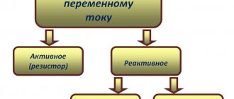
Properties of electromagnetic waves
An electromagnetic wave is an electromagnetic field that varies over time and propagates in space.
The existence of electromagnetic waves was theoretically predicted by the English physicist J. Maxwell in 1864. Electromagnetic waves were discovered by G. Hertz.
The source of an electromagnetic wave is an accelerated moving charged particle - an oscillating charge.
Important! The presence of acceleration is the main condition for the emission of an electromagnetic wave. The greater the acceleration with which the charge moves, the greater the intensity of the emitted wave.
The sources of electromagnetic waves are antennas of various designs, in which high-frequency oscillations are excited.
An electromagnetic wave is called monochromatic if the vectors \( \vec{E} \) and \( \vec{B} \) perform harmonic oscillations with the same frequency (wave frequency).
Electromagnetic wavelength: \( \lambda=cT=\frac{c}{\nu}, \)
where \( c \) is the speed of the electromagnetic wave, \( T \) is the period, \( \nu \) is the frequency of the electromagnetic wave.
Properties of electromagnetic waves
- In a vacuum, an electromagnetic wave propagates with a final speed equal to the speed of light 3·108 m/s.
- Electromagnetic wave is transverse. The oscillations of the intensity vectors of the alternating electric field and the magnetic induction of the alternating magnetic field are mutually perpendicular and lie in a plane perpendicular to the wave speed vector.
- An electromagnetic wave transfers energy in the direction of propagation of the wave.
Important! An electromagnetic wave, unlike a mechanical wave, can propagate in a vacuum.
Flux density or intensity is the electromagnetic energy transferred through a unit area surface per unit time.
The designation is \( I \), the SI unit is watt per square meter (W/m2).
Important! The flux density of electromagnetic wave radiation from a point source decreases in inverse proportion to the square of the distance from the source and is proportional to the fourth power of frequency.
An electromagnetic wave has properties common to all waves, these are:
- reflection,
- refraction,
- interference,
- diffraction,
- polarization.
An electromagnetic wave produces pressure on a substance. This means that the electromagnetic wave has momentum.
Angular (cyclic) frequency of alternating current.
The rotation speed of the radius vector, i.e., the change in the rotation angle within one second, is called the angular (cyclic) frequency of alternating current and is denoted by the Greek letter ? (omega). The angle of rotation of the radius vector at any given moment relative to its initial position is usually measured not in degrees, but in special units - radians.
A radian is the angular value of an arc of a circle, the length of which is equal to the radius of this circle (Figure 2). The entire circle that makes up 360° is equal to 6.28 radians, that is, 2.
Figure 2. Radian.
Then,
1rad = 360°/2
Consequently, the end of the radius vector during one period covers a path equal to 6.28 radians (2). Since within one second the radius vector makes a number of revolutions equal to the frequency of the alternating current f, then in one second its end covers a path equal to 6.28 * f radians. This expression characterizing the rotation speed of the radius vector will be the angular frequency of the alternating current - ?.
So,
?= 6.28*f = 2f
Various types of electromagnetic radiation and their applications
Electromagnetic radiation has wavelengths from 10-12 to 104 m or frequencies from 3·104 to 3·1020.
The following types of electromagnetic radiation are distinguished:
- radio waves;
- infrared radiation;
- visible radiation (light);
- ultraviolet radiation;
- x-ray radiation;
- gamma radiation.
The boundaries between the ranges are arbitrary, but the radiations have qualitative differences in properties. When moving from radiation with a low frequency to radiation with a higher frequency, wave properties appear weaker, and corpuscular (quantum) properties appear stronger.
Radio waves
\( \lambda \) = 103–10-3 m, \( \nu \) = 105–1011 Hz. Sources of radio waves – oscillatory circuit, vibrator.
Radio waves are divided into:
- long (length more than 1 km);
- medium (from 100 m to 1 km);
- short (from 10 to 100 m);
- ultra-short (less than 10 m).
Properties: reflection, absorption, interference, diffraction. Application: radio communications, television, radar.
Radio communication is the transmission of information using radio waves. Radio communication is carried out using modulated radio waves. Modulation of a radio wave is a change in its parameters (amplitude, frequency, initial phase) with a frequency lower than the frequency of the transmitted wave.
The radio communication diagram is shown in the figure:
Transmission of radio waves. The high frequency generator produces high frequency oscillations of the carrier frequency. Sound vibrations enter the microphone, where they are converted into electromagnetic vibrations. In the modulator these oscillations are converted into modulated oscillations. After amplification, the modulated oscillations enter the transmitting antenna, which emits electromagnetic waves. The figure shows a low frequency audio signal and a modulated high frequency signal.
Reception of radio waves. Electromagnetic oscillations enter the receiving antenna and cause electromagnetic oscillations in the receiving circuit. These vibrations enter the amplifier and then the detector. A device with one-way conductivity is used as a detector. It could be a semiconductor diode. In the detector, the signal is demodulated (detected). The detection process consists of separating low (sound) frequency oscillations from high-frequency modulated oscillations. After smoothing and amplification, the signal enters the speaker. The figure shows the detection (demodulation) and smoothing processes.
Radar is the detection and location of objects using radio waves. Radiation is carried out in short pulses. In the time interval between the emission of two successive pulses, the signal reflected from the object is received. Ultrashort radio waves are used for radar.
Infrared (thermal) radiation
\( \lambda \) = 10-3 – 10-7 m, \( \nu \) = 1011 – 1014 Hz. Sources are atoms and molecules of matter.
This radiation is emitted by all bodies at a temperature other than 0 K. Properties: heats a substance when absorbed; interference; diffraction; passes through rain, snow, haze; invisible; refraction, reflection. Application: in night vision devices, in physiotherapy, industry (for drying). Recorded using a thermocouple, bolometer, or photographic method.
Visible radiation
\( \lambda \) = 8·10-7 – 4·10-7 m, \( \nu \) = 4·1011 – 8·1014 Hz.
This radiation is perceived by the eye. Properties: reflection, refraction, absorption, interference, diffraction.
Ultraviolet radiation
\( \lambda \) = 10-8 – 4·10-7 m, \( \nu \) = 8·1014 – 3·1015 Hz. Sources – quartz lamps.
Ultraviolet radiation is produced by luminous mercury vapor and solids with temperatures above 1000°C. Properties: chemical action; high penetrating power; biological effect; invisible. Application: in medicine, industry. Recorded by photographic methods.
X-ray radiation
\( \lambda \) = 10-8 – 10-11 m, \( \nu \) = 3·1016 – 3·1019 Hz. Source: X-ray tubes.
Occurs when fast electrons slow down. Properties: high chemical activity; biological effect; interference; lattice diffraction; high penetrating ability. Application: in medicine, industry, science.
Gamma radiation
The wavelength is less than 10-11 m, frequency is from 1020 Hz and higher. The source is nuclear reactions.
Properties: high penetrating ability, strong biological effect. Application: in medicine, industry (flaw detection), science.
The electromagnetic radiation scale allows us to conclude: all electromagnetic radiation has both wave and quantum properties that complement each other.
Important! Wave properties are more pronounced at low frequencies and long wavelengths, and quantum properties are more pronounced at high frequencies and short wavelengths.
Solving problems on the topic “Electromagnetic oscillations and waves”
Four groups of tasks can be distinguished on this topic:
- to determine the parameters of the oscillatory circuit;
- on the equations of harmonic electromagnetic oscillations;
- to apply Ohm's law;
- to calculate the power and efficiency of the transformer.
The solution to the first group of problems for determining the parameters of an oscillatory circuit is based on the use of Thomson's formula (formula for the period of free electromagnetic oscillations) and the law of conservation and transformation of energy in an oscillatory circuit. Therefore, it is necessary to write down equations for the instantaneous values of the charge and voltage on the capacitor and the current in the coil; write down the equation for the total energy of the oscillatory circuit at an arbitrary moment in time. As additional formulas, you may need formulas for the electrical capacitance of a flat capacitor, the inductance of the coil, and the length of the electromagnetic wave. Remember that the speed of propagation of an electromagnetic wave in a vacuum is equal to the speed of light - 3·108 m/s. In a medium with a refractive index \( n \) the speed of light can be calculated using the formula: \( v=\frac{c}{n}. \)
Important! The amplitude value of the voltage is \( U_m=\frac{q_m}{C} \), the amplitude value of the current is \( I_m=q_m\omega \).
When solving the second group of problems on the equations of harmonic electromagnetic oscillations, it is recommended to write down the equation specified in the problem and the equation of harmonic oscillations in general form. Compare these equations and determine the main characteristics: amplitude, frequency, phase.
When solving problems using Ohm's law, you need to remember that electrical measuring instruments show the effective values of voltage and current. The effective values of the quantities are proportional to the amplitude values. It is important to remember that resonance occurs when inductive and capacitive reactances are equal.
The solution to the fourth group of problems for calculating the power and efficiency of a transformer is based on knowledge of the formulas for efficiency and power in the circuit.
AC phase.
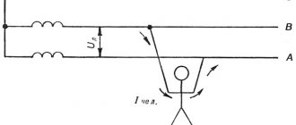
The angle of rotation of the radius vector at any given instant relative to its initial position is called the phase of the alternating current . The phase characterizes the magnitude of the EMF (or current) at a given instant or, as they say, the instantaneous value of the EMF, its direction in the circuit and the direction of its change; phase indicates whether the emf is decreasing or increasing.
Figure 3. AC phase.
A full rotation of the radius vector is 360°. With the beginning of a new revolution of the radius vector, the EMF changes in the same order as during the first revolution. Consequently, all phases of the EMF will be repeated in the same order. For example, the phase of the EMF when the radius vector is rotated by an angle of 370° will be the same as when rotated by 10°. In both of these cases, the radius vector occupies the same position, and, therefore, the instantaneous values of the emf will be the same in phase in both of these cases.
DID YOU LIKE THE ARTICLE? SHARE WITH YOUR FRIENDS ON SOCIAL NETWORKS!
Related materials:
- The concept of alternating current
- Receiving alternating current
- RMS value of current and voltage
- AC current and voltage phase shift
- AC power
Comments
Ruslan_98 10.24.2018 18:22 Well explained. Chewed for ignoramuses like me)
Quote
Ilya_95 09.10.2018 16:27 Thank you, I have been looking for this information for a long time and over long periods. The concepts of period and phase finally became clearer, as if I had managed to get a primeval fire, or figured out how to remove my hand while grabbing a hot frying pan.
Quote
Petya 02/07/2015 17:36 thank you. I hope I can rent
Quote
Update list of comments
Electromagnetic field
An electromagnetic field is a special type of matter through which the electromagnetic interaction of charged bodies or particles occurs.
This concept was introduced by D. Maxwell, who developed Faraday's ideas that an alternating magnetic field generates a vortex electric field.
Any change in the magnetic field generates a vortex electric field in the surrounding space, the lines of force of which are closed. The vortex electric field gives rise to the appearance of a vortex magnetic field, and so on. These alternating electric and magnetic fields, existing simultaneously, form a single electromagnetic field.
The characteristics of this field are the intensity vector and the magnetic induction vector.
If an electric charge is at rest, then only an electric field exists around it.
If the electric field strength is zero and the magnetic induction is non-zero, then only the magnetic field is detected.
If an electric charge moves at a constant speed, then there is an electromagnetic field around it.
Maxwell suggested that with the accelerated movement of charges in space, a disturbance would arise that would propagate in a vacuum at a finite speed. When this disturbance reaches the second charge, the force with which the electromagnetic field acts on this charge will change.
With the accelerated movement of a charge, an electromagnetic wave is emitted. The electromagnetic field is material. It propagates in space in the form of an electromagnetic wave.
If you are already registered, enter your login information!
Previous article Next article
Alternating and direct currents.
Alternating current, in contrast to direct current, continuously changes both in magnitude and direction, and these changes occur periodically, that is, they are exactly repeated at equal intervals of time.
To induce such a current in the circuit, alternating current sources are used, creating an alternating emf that periodically changes in magnitude and direction. Such sources are called alternators.
In Fig. Figure 1 shows a device diagram (model) of a simple alternating current generator.
A rectangular frame made of copper wire is mounted on an axis and rotates in the field of a magnet using a belt drive. The ends of the frame are soldered to copper contact rings, which, rotating with the frame, slide along the contact plates (brushes).
Figure 1. Diagram of a simple alternator
Let us make sure that such a device is indeed a source of alternating EMF.
Let us assume that a magnet creates a uniform magnetic field between its poles, i.e. one in which the density of magnetic field lines in any part of the field is the same. Rotating, the frame intersects the magnetic field lines, and an emf is induced in each of its sides a and b .
Sides c and d of the frame are non-working, since when the frame rotates they do not intersect the magnetic field lines and, therefore, do not participate in the creation of the EMF.
At any moment of time, the EMF arising in side a is opposite in direction to the EMF arising in side b, but in the frame both EMFs act in accordance and in total constitute the total EMF, i.e., induced by the entire frame.
This is easy to verify if you use the well-known right-hand rule to determine the direction of the EMF.
To do this, you need to position the palm of your right hand so that it faces the north pole of the magnet, and the bent thumb coincides with the direction of movement of that side of the frame in which we want to determine the direction of the EMF. Then the direction of the EMF in it will be indicated by the outstretched fingers of the hand.
For whatever position of the frame we determine the direction of the EMF in sides a and b, they always add up and form a total EMF in the frame. In this case, with each revolution of the frame, the direction of the total EMF in it changes to the opposite, since each of the working sides of the frame passes under different poles of the magnet in one revolution.
The magnitude of the EMF induced in the frame also changes, as the speed at which the sides of the frame intersect the magnetic field lines changes. Indeed, at the time when the frame approaches its vertical position and passes it, the speed of intersection of the force lines by the sides of the frame is greatest, and the largest EMF is induced in the frame. At those moments in time when the frame passes its horizontal position, its sides seem to slide along the magnetic lines of force without crossing them, and no emf is induced.
Thus, with uniform rotation of the frame, an emf will be induced in it, periodically changing both in magnitude and direction.
The EMF arising in the frame can be measured with a device and used to create a current in an external circuit.
Using the phenomenon of electromagnetic induction, it is possible to obtain an alternating emf and, therefore, an alternating current.
Alternating current for industrial purposes and for lighting is produced by powerful generators driven by steam or water turbines and internal combustion engines.
Graphic representation of direct and alternating currents
The graphical method makes it possible to visually represent the process of changing a particular variable depending on time.
The construction of graphs of variables that change over time begins with the construction of two mutually perpendicular lines, called the axes of the graph. Then, segments of time are plotted on the horizontal axis on a certain scale, and on the vertical axis, also on a certain scale, the values of the quantity whose graph is going to be plotted (EMF, voltage or current).
In Fig. 2 graphically shows direct and alternating currents. In this case, we plot the current values, and vertically up from the point of intersection of the O axes we plot the current values of one direction, which is usually called positive, and down from this point - in the opposite direction, which is usually called negative.
Figure 2. Graphical representation of DC and AC current
Point O itself serves simultaneously as the beginning of the countdown of current values (vertically down and up) and time (horizontally to the right). In other words, this point corresponds to the zero value of the current and the initial moment in time from which we intend to trace how the current will change in the future.
Let us verify the correctness of what is constructed in Fig. 2, and a graph of a constant current of 50 mA.
Since this current is constant, i.e., does not change its magnitude and direction over time, the same current values, i.e., 50 mA, will correspond to different moments in time. Therefore, at a time equal to zero, i.e. at the initial moment of our observation of the current, it will be equal to 50 mA. By plotting upward on the vertical axis a segment equal to the current value of 50 mA, we get the first point of our graph.
We must do the same for the next moment in time, corresponding to point 1 on the time axis, i.e., set aside a segment vertically upward from this point, also equal to 50 mA. The end of the segment will determine the second point of the graph.
Having done a similar construction for several subsequent moments in time, we will obtain a series of points, the connection of which will give a straight line, which is a graphical representation of a direct current of 50 mA.
Plotting a graph of the EMF variable
Let's now move on to studying the graph of the EMF variable. In Fig. 3 at the top shows a frame rotating in a magnetic field, and at the bottom is a graphical representation of the emerging EMF variable.
Figure 3. Plotting a graph of the variable EMF
Let's begin to uniformly rotate the frame clockwise and follow the progress of the change in the EMF in it, taking the horizontal position of the frame as the initial moment.
At this initial moment, the EMF will be zero, since the sides of the frame do not intersect the magnetic lines of force. On the graph, this zero EMF value corresponding to the moment t = 0 will be represented by point 1.
With further rotation of the frame, an emf will begin to appear in it and will increase in magnitude until the frame reaches its vertical position. On the graph, this increase in EMF will be depicted as a smooth upward curve that reaches its peak (point 2).
As the frame approaches the horizontal position, the emf in it will decrease and drop to zero. On the graph this will be depicted as a descending smooth curve. Consequently, during the time corresponding to half a revolution of the frame, the EMF in it managed to increase from zero to its maximum value and again decrease to zero (point 3).
With further rotation of the frame, an emf will again arise in it and will gradually increase in magnitude, but its direction will already change to the opposite, which can be verified by applying the right-hand rule.
The graph takes into account the change in the direction of the EMF in that the curve depicting the EMF intersects the time axis and is now located below this axis. The EMF increases again until the frame takes a vertical position. Then the EMF will begin to decrease, and its value will become equal to zero when the frame returns to its original position, having completed one full revolution. On the graph this will be expressed by the fact that the EMF curve, having reached its peak in the opposite direction (point 4), then meets the time axis (point 5).
This ends one cycle of changing the EMF, but if we continue to rotate the frame, a second cycle immediately begins, exactly repeating the first, which, in turn, will be followed by a third, and then a fourth, and so on until we stop the rotation framework.
Thus, for each revolution of the frame, the EMF arising in it completes a full cycle of its change.
If the frame is closed to any external circuit, then an alternating current will flow through the circuit, the graph of which will be the same in appearance as the EMF graph.
The wave-like curve we obtained is called a sine wave, and the current, EMF or voltage that changes according to this law are called sinusoidal.
The curve itself is called a sine wave because it is a graphical representation of a variable trigonometric quantity called sine.
The sinusoidal nature of current change is the most common in electrical engineering, therefore, when speaking about alternating current, in most cases we mean sinusoidal current.
To compare different alternating currents (EMF and voltages), there are quantities that characterize a particular current. These are called AC parameters.
Period, amplitude and frequency - parameters of alternating current
Alternating current is characterized by two parameters - period and amplitude, knowing which we can judge what kind of alternating current it is and build a current graph.
Figure 4. Sinusoidal current curve
The period of time during which a complete cycle of current change occurs is called a period. The period is designated by the letter T and is measured in seconds.
The period of time during which half of the complete cycle of current change occurs is called a half-cycle. Consequently, the period of change of current (EMF or voltage) consists of two half-cycles. It is quite obvious that all periods of the same alternating current are equal to each other.
As can be seen from the graph, during one period of its change the current reaches twice its maximum value.
The maximum value of an alternating current (emf or voltage) is called its amplitude or amplitude current value.
Im, Em and Um are generally accepted designations for the amplitudes of current, emf and voltage.
We first of all paid attention to the amplitude value of the current, however, as can be seen from the graph, there are countless intermediate values that are less than the amplitude value.
The value of alternating current (EMF, voltage) corresponding to any selected moment in time is called its instantaneous value.
i, e and u are generally accepted designations for instantaneous values of current, emf and voltage.
The instantaneous current value, as well as its amplitude value, can be easily determined using a graph. To do this, from any point on the horizontal axis corresponding to the moment of time we are interested in, we draw a vertical line to the point of intersection with the current curve; the resulting segment of the vertical straight line will determine the value of the current at a given moment, i.e. its instantaneous value.
It is obvious that the instantaneous value of the current after time T/2 from the starting point of the graph will be equal to zero, and after time T/4 its amplitude value. The current also reaches its amplitude value; but in the opposite direction, after a time equal to 3/4 T.
So, the graph shows how the current in the circuit changes over time, and that each moment in time corresponds to only one specific value of both the magnitude and direction of the current. In this case, the value of the current at a given moment in time at one point in the circuit will be exactly the same at any other point in this circuit.
The number of complete periods performed by the current in 1 second is called the frequency of alternating current and is denoted by the Latin letter f.
To determine the frequency of alternating current, i.e., to find out how many periods of change the current has completed within 1 second, it is necessary to divide 1 second by the time of one period f = 1/T. Knowing the frequency of the alternating current, you can determine the period: T = 1/f
The frequency of alternating current is measured in a unit called the hertz.
If we have an alternating current whose frequency is 1 hertz, then the period of such current will be equal to 1 second. And, conversely, if the period of current change is 1 second, then the frequency of such current is 1 hertz.
So, we have determined the parameters of alternating current - period, amplitude and frequency - which allow us to distinguish different alternating currents, emfs and voltages from each other and build their graphs when necessary.
When determining the resistance of various circuits to alternating current, use another auxiliary quantity that characterizes alternating current, the so-called angular or circular frequency.
The circular frequency is denoted by the letter ω and is related to the frequency f by the relation ω = 2πf
Let us explain this dependence. When constructing a graph of the variable EMF, we saw that during one full revolution of the frame, a complete cycle of EMF changes occurs. In other words, in order for the frame to make one revolution, i.e., turn 360°, it takes time equal to one period, i.e. T seconds. Then in 1 second the frame makes a 360°/T revolution. Therefore, 360°/T is the angle through which the frame rotates in 1 second, and expresses the speed of rotation of the frame, which is usually called angular or circular speed.
But since the period T is related to the frequency f by the ratio f = 1/T, the circular speed can be expressed in terms of frequency and will be equal to ω = 360°f.
So, we came to the conclusion that ω = 360°f. However, for the convenience of using the circular frequency in all kinds of calculations, the angle of 360° corresponding to one revolution is replaced by a radial expression equal to 2π radians, where π = 3.14. Thus, we finally obtain ω = 2πf. Therefore, to determine the circular frequency of alternating current (emf or voltage), the frequency in hertz must be multiplied by a constant number 6.28.
Source of information: “School for an electrician: electrical engineering and electronics”
Previous article Next article
Quasi-stationary condition
In the case of alternating current, one subtle point arises. Let's assume that the circuit consists of several elements connected in series.
If the source voltage changes according to a sinusoidal law, then the current strength does not have time to instantly take on the same value throughout the entire circuit - it takes some time to transfer interactions between charged particles along the circuit.
Meanwhile, as in the case of direct current, we would like to consider the current strength to be the same in all elements of the circuit. Fortunately, in many practically important cases we actually have the right to do this.
Let's take, for example, alternating voltage frequency Hz (this is the industrial standard in Russia and many other countries). Voltage fluctuation period: s.
The interaction between charges is transmitted at the speed of light: m/s. In a time equal to the oscillation period, this interaction will spread over a distance:
m km.
Therefore, in cases where the length of the circuit is several orders of magnitude less than this distance, we can neglect the propagation time of the interaction and assume that the current strength instantly takes on the same value throughout the entire circuit.
Now consider the general case when the voltage oscillates with a cyclic frequency. The period of oscillation is equal, and during this time the interaction between charges is transmitted over a distance. Let be the length of the chain. We can neglect the interaction propagation time if much less:
(2)
Inequality (2) is called the quasi-stationarity condition
.
When this condition is met, we can assume that the current strength in the circuit instantly takes on the same value throughout the entire circuit. Such a current is called quasi-stationary
.
In what follows we assume that the alternating current changes slowly enough that it can be considered quasi-stationary. Therefore, the current strength in all series-connected elements of the circuit will take the same value - its own at each moment of time. It is called the instantaneous current value
.