Hello, my friend, are you interested in learning everything about the Kirchhoff method, then read to the end with inspiration. In order to better understand what the Kirchhoff method, Kirchhoff's law is, I strongly recommend reading everything from the category Electrical engineering, Circuit design, Analog devices.
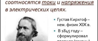
In complex electrical circuits, that is, where there are several different branches and several sources of EMF, a complex distribution of currents also occurs. However, with known values of all the emfs and resistances of the resistive elements in the circuit, we can clear the values of these currents and their direction in any circuit circuit using Kirchhoff's first and second laws . The rules were formulated in 1845; this is not Kirchhoff’s only discovery. Kirchhoff and Bunsen actively studied the emission spectra of chemical elements using Fraunhofer's inventions. Using a prism or diffraction grating, the light was split into spectral components, and scientists observed the effect. This is how the individual frequencies of a number of elements in the periodic table were established. These scientists laid the foundations of spectroscopy. Kirchhoff devoted a lot of time to various branches of science. For example, I found an error in setting the boundary conditions for solving differential equations for membrane vibrations, presented to the public in 1811 by Sophie Germain. One should not think that the phrase Kirchhoff's law is narrowly limited to two rules, one of which directly leads to Ohm's law formulated earlier.
| German Gustav Robert Kirchhoff | |
| Date of Birth | March 12, 1824 |
An example of a complex electrical circuit can be seen in Figure 1.
Figure 1. Complex electrical circuit.
Sometimes Kirchhoff's laws are called Kirchhoff's rules , especially in older literature.
So, to begin with, let me remind you of the essence of Kirchhoff’s first and second laws, and then consider examples of calculating currents and voltages in electrical circuits, with practical examples and answers to questions that were asked to me in the comments on the site.
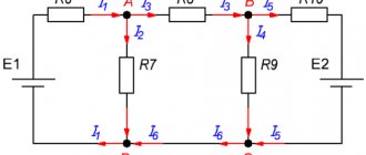
The most accurate method, but with its help you can determine the parameters of a circuit with a small number of circuits (1-3). Algorithm: 1. Determine the number of nodes q, branches p and independent circuits; 2. Set the directions of currents and circuit bypasses arbitrarily; 3. Establish the number of independent equations according to Kirchhoff’s 1st law (q - 1) and compose them, where q is the number of nodes; 4. Determine the number of equations according to Kirchhoff’s 2nd law (p – q + 1) and compose them; 5. Solving the equations together, we determine the missing parameters of the circuit; 6. Based on the data received, the calculations are checked by substituting the values into the equations according to Kirchhoff’s 1st and 2nd laws or by compiling and calculating the power balance. Example:
Fig. 1. According to the proposed algorithm, we determine the number of nodes and branches of the circuit in Fig. 1 q = 3, p = 5, therefore, there are 2 equations according to Kirchhoff’s 1st law, and there are 3 equations according to Kirchhoff’s 2nd law. Let’s write these equations according to the rules:
Let's create the power balance equations:
Kirchhoff's rules and laws
Kirchhoff's rules (often called Kirchhoff's Laws in technical literature) are relationships that hold between currents and voltages in sections of any electrical circuit.
Solutions of systems of linear equations compiled on the basis of Kirchhoff's rules make it possible to find all currents and voltages in electrical circuits of direct, alternating and quasi-stationary current.
They are of particular importance in electrical engineering because of their versatility, as they are suitable for solving many problems in the theory of electrical circuits and practical calculations of complex electrical circuits.
Application of Kirchhoff's rules to a linear electrical circuit allows us to obtain a system of linear equations for currents or voltages and, accordingly, when solving this system, find the current values on all branches of the circuit and all internodal voltages.
Formulated by Gustav Kirchhoff in 1845.
The name “Rules” is more correct because these rules are not fundamental laws of nature, but follow from the fundamental laws of conservation of charge and irrotation of the electrostatic field (Maxwell’s third equation with a constant magnetic field). These rules should not be confused with two other Kirchhoff laws in chemistry and physics.
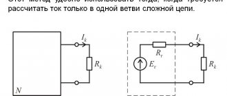
Loop current method
The method of calculating electrical circuits discussed above when analyzing large and branched circuits leads to unreasonably labor-intensive calculations, and therefore is rarely used. The loop current method is more widely used, allowing a significant reduction in the number of equations. In this case, instead of currents in the branches of an electrical circuit, the so-called loop currents are determined using Kirchhoff’s second law. Thus, the number of required equations will be equal to the number of independent circuits. As an example, let's calculate the circuit shown in the figure below.
Circuit calculation using the loop current method.
If we were to calculate the circuit using the method of Ohm's and Kirchhoff's laws, then it would be necessary to solve a system of five equations. To calculate using the loop current method, only three equations are needed.
At the beginning of the calculation, independent contours are identified, in our case these are: E1R1R2E2, E2R2R4E3R3 and E3R4R5. Then the circuits are assigned an arbitrarily directed circuit current, which has the same direction for all sections of the selected circuit; in our case, for the first circuit the circuit current will be Ia, for the second - Ib, for the third - Ic. As can be seen from the figure, some loop currents correspond to currents in the branches
The remaining currents can be found as the difference between two loop currents
As a result of the choice of loop currents, it is possible to create a system of equations according to Kirchhoff’s second law
Let's calculate the circuit shown in the figure above with the following parameters E1 = E3 = 100 V, E2 = 50 V, R1 = R2 = 10 Ohm, R3 = R4 = R5 = 20 Ohm. Let's write the system of equations
As a result of solving the system, we obtain Ia = I1 = 4.286 A, Ib = I3 = 3.571 A, Ic = I5 = -0.714 A, I2 = -0.715 A, I4 = 4.285 A. Just like in the previous case, if the currents are negative, This means that the actual direction is opposite to the accepted one. Thus, the currents I2 and I5 have the opposite direction to those shown in the figure.
Kirchhoff's first law
Formulation No. 1: The sum of all currents flowing into a node is equal to the sum of all currents flowing out of the node.
Formulation No. 2: The algebraic sum of all currents in a node is equal to zero.
Online demonstration and simulation of the Kirchhoff method: Open full screen
Let us explain Kirchhoff's first law using the example of Figure 2.
Figure 2. Electrical circuit assembly.
Here the current I1 is the current flowing into the node, and the currents I2 and I3 are the currents flowing out of the node. Then, using formulation No. 1, we can write:
I1 = I2 + I3 (1)
To confirm the validity of formulation No. 2, we transfer the currents I2 and I 3 to the left side of expression (1) , thereby obtaining:
I1 - I2 - I3 = 0 (2)
The minus signs in expression (2) mean that currents flow out of the node.
The signs for inflowing and outflowing currents can be taken arbitrarily, however, in general, inflowing currents are always taken with a “+” sign, and outflowing currents with a “-” sign (for example, as happened in the expression (2)).
Calculation of electrical circuits online
A program has appeared on the website for calculating steady-state conditions of electrical circuits according to the laws of TOE. At the moment, calculation methods have been implemented using Ohm's laws, Kirchhoff's laws, the nodal potential method, the loop current method, and the equivalent generator method. The program also allows you to calculate the equivalent resistance of the circuit relative to the power source. The program allows you to draw a diagram, set the parameters of its elements and calculate the diagram. As a result, a text description of the calculation procedure is generated, the power balance is calculated and vector diagrams are constructed.
Drawing a diagram is done by drag-and-dropping elements from the sidebar and then connecting the selected elements.
The following elements with configurable parameters are available in the sidebar:
- resistor: element number;
- resistance, Ohm;
- item number;
- item number;
- item number;
- item number;
Instructions for using the program are given here.
Calculation methods
After completing drawing the diagram, clicking the “Calculation” button starts the calculation of the electrical circuit. The program analyzes the source circuit and if any errors are detected, it reports this. Upon successful analysis of the circuit, the calculation using TOE methods is started.
Calculation according to Ohm's law
Calculation according to Ohm's law is carried out for single-circuit circuits. The calculation method used is given here.
Example diagram and calculation:
Initial data and diagram:
- E1: Item number: 1
- Amplitude value: 100 V
- Initial phase: 0
- Item number: 1
After clicking the “Calculation” button, a solution is generated:
The original circuit has only one circuit. Let's calculate it using Ohm's law.
According to Ohm's law, the current in a closed circuit is equal to the ratio of the circuit's emf to the resistance. Let's create an equation, taking the positive direction of the current $ \underline{I} $ to be the direction of the EMF source $ \underline{E}_{1} $:
$$ R_{1}\cdot \underline{I} = \underline{E}_{1} $$
Let us substitute the values of resistances and sources into the resulting system of equations and obtain:
$$ 1.0\cdot \underline{I}=100 $$
Hence the required current in the circuit is equal to
$$ \underline{I} = 100\space \textrm{A}$$
Calculation according to Kirchhoff's laws
For multi-circuit circuits, the calculation is carried out according to Kirchhoff's laws. The calculation method used is given here.
Example diagram and calculation:
Initial data and diagram:
- E1: Item number: 1
- Amplitude value: 100 V
- Initial phase: 0
- Item number: 1
- Item number: 1
- Item number: 1
After clicking the “Calculation” button, the numbering of nodes appears on the original diagram and a solution is generated:
Let's calculate the circuit using Kirchhoff's laws.
In this scheme: nodes - 2, branches - 3, independent circuits - 2.
Let us arbitrarily set the directions of currents in the branches and the directions of traversal of the circuits.
Accepted directions of currents: Current $ \underline{I}_{1} $ is directed from node '2 y.' to node '1 y.' through the elements $ \underline{E}_{1} $, $ R_{1} $. Current $ \underline{I}_{2} $ is directed from node '1 y.' to node '2 y.' through the elements of $L_{1}$. Current $ \underline{I}_{3} $ is directed from node '1 y.' to node '2 y.' through the elements of $C_{1}$.
Accepted directions for traversing contours: Contour No. 1 is traversed through the elements $ \underline{E}_{1} $, $ R_{1} $, $ L_{1} $ in the specified order. Circuit No. 2 is traversed through the elements $ L_{1} $, $ C_{1} $ in the specified order.
Let's create equations according to Kirchhoff's first law. When drawing up equations, we will take currents “flowing” into a node with a “+” sign, and “outgoing” ones with a “−” sign.
The number of equations compiled according to Kirchhoff's first law is equal to $ N_\textrm{y} − 1 $, where $ N_\textrm{y} $ is the number of nodes. For this scheme, the number of equations according to Kirchhoff’s first law is 2 − 1 = 1.
Let's create an equation for node No. 1:
$$ \underline{I}_{1} − \underline{I}_{2} − \underline{I}_{3} = 0 $$
Let's create equations using Kirchhoff's second law. When drawing up equations, positive values for currents and EMF are selected if they coincide with the direction of traversal of the circuit.
The number of equations compiled according to Kirchhoff's second law is equal to $ N_\textrm{в} − N_\textrm{у} + 1 $, where $ N_\textrm{в} $ is the number of branches. For this scheme, the number of equations according to Kirchhoff’s second law is 3 − 2 + 1 = 2.
Let's create an equation for circuit No. 1:
$$ R_{1}\cdot \underline{I}_{1} + jX_{L1}\cdot \underline{I}_{2}=\underline{E}_{1} $$
Let's create an equation for circuit No. 2:
$$ jX_{L1}\cdot \underline{I}_{2} − (−jX_{C1})\cdot \underline{I}_{3}=0 $$
Let us combine the resulting equations into one system, and at the same time transfer the known quantities to the right side, leaving only the components with the required currents on the left side. The system of equations according to Kirchhoff’s laws for the original circuit is as follows:
$$ \begin{cases}\underline{I}_{1} − \underline{I}_{2} − \underline{I}_{3} = 0 \\ R_{1}\cdot \underline{I }_{1}+jX_{L1}\cdot \underline{I}_{2} = \underline{E}_{1} \\ jX_{L1}\cdot \underline{I}_{2}−( −jX_{C1})\cdot \underline{I}_{3} = 0 \\ \end{cases} $$
Let us substitute the values of resistances and sources into the resulting system of equations and obtain:
$$ \begin{cases}\underline{I}_{1} − \underline{I}_{2} − \underline{I}_{3}=0 \\ \underline{I}_{1}+ j \cdot \underline{I}_{2}=100 \\ j \cdot \underline{I}_{2}+ j \cdot \underline{I}_{3}=0 \\ \end{cases} $$
Let us solve the system of equations and obtain the required currents:
$$ \underline{I}_{1} = 0 $$
$$ \underline{I}_{2} = −100j $$
$$ \underline{I}_{3} = 100j $$
Recommended Posts
- Calculation of electrical circuits using the method of nodal potentials: conclusion of the method
Along with solving electrical circuits according to Kirchhoff’s laws and the method of loop currents, the method of nodal... - Kirchhoff's laws for calculating electrical circuits When calculating electrical circuits, including for modeling purposes, Kirchhoff's laws are widely used, allowing...
- Vector diagrams of electrical circuits When studying electrical circuits and modeling, vector diagrams of currents and voltages are often used. Under the vector...
Kirchhoff's second law.
Formulation: The algebraic sum of the EMF acting in a closed circuit is equal to the algebraic sum of the voltage drops across all resistive elements in this circuit.
Online demonstration and simulation of the Kirchhoff method: Open full screen
Here the term “algebraic sum” means that both the magnitude of the EMF and the magnitude of the voltage drop across the elements can be either with a “+” or a “-” sign. In this case, the sign can be determined using the following algorithm:
1. Select the direction of traversing the contour (two options, either clockwise or counterclockwise).
2. We arbitrarily select the direction of currents through the circuit elements.
3. We arrange signs for the EMF and voltages falling on the elements according to the rules:
— EMF that creates a current in the circuit, the direction of which coincides with the direction of bypassing the circuit, is written with a “+” sign, otherwise the EMF is written with a “-” sign.
— voltages falling across the circuit elements are recorded with a “+” sign if the current flowing through these elements coincides in the direction of bypassing the circuit, otherwise the voltages are recorded with a “-” sign.
For example, consider the circuit shown in Figure 3 and write the expression according to Kirchhoff's second law, going around the circuit clockwise and choosing the direction of the currents through the resistors, as shown in the figure.
Figure 3. The website https://intellect.icu talks about this. Electric circuit to explain Kirchhoff's second law.
E1- E2 = -UR1 - UR2 or E1 = E2 - UR1 - UR2 (3)
Kirchhoff's first rule
Gustav Kirchhoff's first rule is formulated based on the law of conservation of charge. The physicist understood that the charge cannot be retained in the node, but is distributed along the branches of the circuit that form this connection.
Kirchhoff assumed, and subsequently substantiated on the basis of experiments, that the number of charges entering the node is the same as the amount of current flowing out of it.
Figure 1 shows a simple circuit diagram. Points A, B, C, D indicate the contour nodes in the center of the diagram.
Rice. 1. Circuit diagram
Current I1 enters node A, formed by the branches of the circuit. In the diagram, the electric charge is distributed in two directions - along branches AB and AD. According to Kirchhoff's rule, the incoming current is equal to the sum of the outgoing ones: I1 = I2 + I3.
Figure 2 shows an abstract node, along the branches of which current flows in different directions. If you add the vectors i1, i2, i3, i4, then, according to Kirchhoff’s first rule, the vector sum will be equal to 0: i1 + i2 + i3 + i4 = 0. There can be as many branches as you like, but the equality will always be fair, taking into account the direction of the vectors .
Rice. 2. Abstract node
Let us write our conclusions in algebraic form for the general case:
To use this formula, you need to take into account the signs. To do this, you need to select the direction of one of the current vectors (no matter which one) and designate it with a plus sign. In this case, the signs of all other quantities are determined based on their direction in relation to the selected vector.
To avoid confusion, the current directed to the node point is considered positive, and the vectors directed from the node are considered negative.
Let us state Kirchhoff’s first rule, expressed by the above formula: “The algebraic sum of the currents converging in a certain node is equal to zero, if we consider the incoming currents to be positive and the outgoing currents to be negative.”
The first rule complements the second rule formulated by Kirchhoff. Let's move on to consider it.
On the significance for electrical engineering
Kirchhoff's rules are of an applied nature and allow, along with and in combination with other techniques and methods (equivalent generator method, superposition principle, method of drawing up a potential diagram) to solve electrical engineering problems. Kirchhoff's rules have found wide application due to the simplicity of the formulation of equations and the possibility of solving them using standard methods of linear algebra (Cramer's method, Gauss's method, etc.).
Kirchhoff's radiation law
Kirchhoff's radiation law states that the ratio of the emissivity of any body to its absorption capacity is the same for all bodies at a given temperature for a given frequency for equilibrium radiation and does not depend on their shape, chemical composition, etc.
In its modern formulation, the law reads as follows:
The ratio of the emissivity of any body to its absorption capacity is the same for all bodies at a given temperature for a given frequency and does not depend on their shape and chemical nature.
It is known that when electromagnetic radiation falls on a certain body, part of it is reflected, part is absorbed, and part can be transmitted. The fraction of radiation absorbed at a given frequency is called the body's absorptivity. On the other hand, every heated body emits energy according to a certain law called the emissivity of the body.
The values of and can vary greatly when moving from one body to another, however, according to Kirchhoff’s law of radiation, the ratio of emissivity and absorption abilities does not depend on the nature of the body and is a universal function of frequency (wavelength) and temperature:
By definition, an absolutely black body absorbs all radiation incident on it, that is, for it. Therefore, the function coincides with the emissivity of a completely black body, described by Planck’s formula, as a result of which the emissivity of any body can be found based only on its absorption capacity.
Real bodies have an absorption capacity of less than unity, and therefore an emissivity less than that of an absolutely black body. Bodies whose absorption capacity does not depend on frequency are called gray. Their spectrum has the same appearance as that of a completely black body. In the general case, the absorption capacity of bodies depends on frequency and temperature, and their spectrum can differ significantly from the spectrum of an absolutely black body. The study of the emissivity of different surfaces was first carried out by the Scottish scientist Leslie using his own invention - the Leslie cube.
In theoretical studies, it is more convenient to use the frequency function to characterize the spectral composition of equilibrium thermal radiation. In experimental work, it is more convenient to use the wavelength function. Both functions are related to each other by the formula
In astrophysics, Kirchhoff's law is often used in the following form:
,
where is the emissivity (energy emitted by a unit volume in a unit frequency interval per unit solid angle per unit time); is the absorption coefficient taking into account stimulated emission (, where is the density of the substance, and and are, respectively, the opacity and effective path length of photons for frequency ); is the intensity of blackbody radiation.
Kirchhoff's law is valid only for cases of thermal equilibrium. However, it is often used for nonequilibrium systems, when the radiation is not in equilibrium with matter and its frequency distribution differs significantly from the Planck one. In this case, often (but not always) the assumption of thermodynamic equilibrium between the particles of the emitting substance turns out to be a good approximation. The degree of deviation from Kirchhoff's law can serve as a measure of the difference between the radiation of space objects and thermal radiation.
Kirchhoff's law for a magnetic circuit
The use of independent equations is also possible when calculating magnetic circuits. The Kirchhoff rules formulated above are also valid for calculating the parameters of magnetic fluxes and magnetizing forces.
Rice. 4. Magnetic circuits
In particular: ∑Ф=0.
That is, for magnetic fluxes, Kirchhoff’s first rule can be expressed in the words: “The algebraic sum of all possible magnetic fluxes relative to a node of a magnetic circuit is equal to zero.
Let us formulate the second rule for magnetizing forces F: “In a closed magnetic circuit, the algebraic sum of magnetizing forces is equal to the sum of magnetic stresses.” This statement is expressed by the formula: ∑F=∑U or ∑Iω = ∑НL, where ω is the number of turns, H is the magnetic field strength, and the symbol L denotes the length of the center line of the magnetic circuit. (It is conventionally assumed that each point of this line coincides with the lines of magnetic induction).
The second rule used to calculate magnetic circuits is nothing more than an alternative form of representing the total current law.
Note: When composing equations using formulas arising from Kirchhoff's rules, one must first determine the positive direction of the flows operating in the branches, comparing them with the direction of the bypasses of existing circuits.
When the magnetic flux vectors coincide with the bypass directions (in some sections), we take the voltage drop on these branches with the “+” sign, and those counter to it with the “–” sign.
Kirchhoff's law in chemistry
Kirchhoff's law states that the temperature coefficient of the thermal effect of a chemical reaction is equal to the change in the heat capacity of the system during the reaction.
Differential form of the law:
Integral form of the law:
where and are the isobaric and isochoric heat capacities, is the difference in the isobaric heat capacities of the reaction products and the starting substances, is the difference in the isochoric heat capacities of the reaction products and the starting substances, and and are the corresponding thermal effects.
If the difference is small, then we can accept and, accordingly, the integral form of the equations will take the following form:
With a large temperature difference, it is necessary to take into account the temperature dependences of the heat capacities: and
see also
- two node method,
- analysis of sinusoidal current circuits, Ohm's law in complex form,
- two node method,
- Thevenin's theorem,
- Norton's theorem,
- Ohm's law for a section of a circuit, Ohm's law,
Do you like the Kirchhoff method? or do you have any useful tips and additions? Write to other readers below. I hope that now you understand what the Kirchhoff method, Kirchhoff’s law is and why all this is needed, and if you don’t understand, or if you have any comments, then don’t hesitate to write or ask in the comments, I will be happy to answer. In order to gain a deeper understanding, I strongly recommend studying all the information from the category Electrical Engineering, Circuit Engineering, Analog Devices
Write answers to questions for self-test in the comments, we will check, or ask your own question on this topic.
1.10. Kirchhoff's rules for branched chains
To simplify the calculations of complex electrical circuits containing inhomogeneous sections, Kirchhoff's rules are used, which are a generalization of Ohm's law for the case of branched circuits.
In branched circuits, nodal points (nodes) can be identified at which at least three conductors converge (Fig. 1.10.1). Currents flowing into a node are considered positive; flowing from the node – negative.
| Figure 1.10.1. Electrical circuit assembly. I1, I2 > 0; I3, I4 < 0 |
Charge accumulation cannot occur in the nodes of a DC circuit. This leads to Kirchhoff's first rule:
The algebraic sum of the current strengths for each node in a branched circuit is equal to zero:
| I1 + I2 + I3 + … + In = 0. |
Kirchhoff's first rule is a consequence of the law of conservation of electric charge.
In a branched chain, it is always possible to distinguish a certain number of closed paths, consisting of homogeneous and heterogeneous sections. Such closed paths are called contours. Different currents can flow in different parts of the selected circuit. In Fig. Figure 1.10.2 shows a simple example of a branched chain. The circuit contains two nodes a and d, in which identical currents converge; therefore only one of the nodes is independent (a or d).
| Figure 1.10.2. An example of a branched electrical circuit. The circuit contains one independent node (a or d) and two independent circuits (for example, abcd and adef) |
In the circuit, three circuits abcd, adef and abcdef can be distinguished. Of these, only two are independent (for example, abcd and adef), since the third does not contain any new regions.
Kirchhoff's second rule is a consequence of Ohm's generalized law.
Let us write down a generalized Ohm's law for the sections that make up one of the contours of the circuit shown in Fig. 1.10.2, for example abcd. To do this, in each section you need to set the positive direction of the current and the positive direction of bypassing the circuit. When writing the generalized Ohm's law for each of the sections, it is necessary to observe certain “sign rules”, which are explained in Fig. 1.10.3.
| Figure 1.10.3. "Sign Rules" |
For contour sections abcd, the generalized Ohm's law is written as:
For section bc: I1R1 = Δφbc – 1.
For section da: I2R2 = Δφda – 2.
Adding the left and right sides of these equalities and taking into account that Δφbc = – Δφda, we obtain:
| I1R1 + I2R2 = Δφbc + Δφda – 1 + 2 = –1 – 2. |
Similarly, for the adef contour one can write:
| – I2R2 + I3R3 = 2 + 3. |
Kirchhoff's second rule can be formulated as follows: the algebraic sum of the products of the resistance of each section of any closed circuit of a branched DC circuit and the current strength in this section is equal to the algebraic sum of the emf along this circuit.
The first and second Kirchhoff rules, written for all independent nodes and circuits of a branched circuit, together provide the necessary and sufficient number of algebraic equations for calculating the values of voltages and currents in an electrical circuit. For the circuit shown in Fig. 1.10.2, the system of equations for determining three unknown currents I1, I2 and I3 has the form:
| I1R1 + I2R2 = – 1 – 2, |
| – I2R2 + I3R3 = 2 + 3, |
| – I1 + I2 + I3 = 0. |
Thus, Kirchhoff's rules reduce the calculation of a branched electrical circuit to solving a system of linear algebraic equations. This solution does not cause any fundamental difficulties, however, it can be very cumbersome even in the case of fairly simple circuits. If, as a result of the solution, the current strength in some area turns out to be negative, then this means that the current in this area goes in the direction opposite to the selected positive direction.
| Model. DC circuits |
| Model. Capacitors in DC circuits |