TOE › Calculation of DC circuits
When calculating the operating mode of an electrical circuit, it is very often necessary to determine the currents, voltages and powers in all its sections for given EMF sources and resistances of the circuit sections. This calculation is based on the application of Kirchhoff's laws.
This article assumes that you are familiar with the definitions of node, branch, and loop.
Kirchhoff's first law
Kirchhoff's first law states that in the branches forming a node of an electrical circuit, the algebraic sum of currents is equal to zero (currents entering the node are considered positive, currents leaving the node are considered negative).
Using this law for node A (Figure 1), we can write the following expression:
Figure 1 - Kirchhoff's first law
I1 + I2 − I3 + I4 − I5 − I6 = 0.
Try to apply Kirchhoff's first law yourself to determine the current in a branch. The diagram above shows six branches forming an electrical node B , the currents of the branches enter and exit the node. One of the currents i is unknown.
#1. Write down the expression for node B
Wrong
Further
#2. Find the current i
Wrong
Complete
Example
Suppose an electrical network consists of two voltage sources and three resistors.
According to the first law:
i1-i2-i3={\displaystyle i_{1}-i_{2}-i_{3}=0\,}
Application of the second law to a closed circuit s
1 and replacing the voltage using Ohm's law gives
: = 0}
Second law, again combined with Ohm's law, applied to a closed circuit s
2, gives:
-r3i3-E2-E1+r2i2={\displaystyle -R_{3}i_{3}-{\mathcal {E))_{2}-{\mathcal {E))_{1}+ R_{2} i_{2} = 0}
This leads to a system of linear equations in I
1 ,
I
2 ,
I
3 :
{i1-i2-i3=-p2i2+E1-p1i1=-p3i3-E2-E1+p2i2={\displaystyle {\begin {cases} i_{1}-i_{2}- i_{3}&=0\\-R_{2}i_{2}+{\mathcal {E}}_{1}-R_{1}i_{1}&=0\\-R_{3}i_ {3} - {\mathcal {E}}_{2} - {\mathcal {E}}_{1}+R_{2}i_{2}&=0\end{cases}}}
which is equivalent
{i1+(-i2)+(-i3)=E1+E2+(-i3)=E1+E2{\displaystyle {\begin {cases} i_{1}+(-i_{2})+(-i_ {3})&=0\\R_{1}i_{1}+R_{2}i_{2}+0i_{3}&={\mathcal {E}}_{1}\\0i_{1} +R_{2}i_{2}-R_{3}i_{3}&={\mathcal {E}}_{1}+{\mathcal {E}}_{2}\end{case))}
Assuming
R1=100Ω, R2=200Ω, R3=300Ω{\displaystyle R_{1}=100\Omega,\R_{2}=200\Omega,\R_{3}=300\Omega} E1=3V,E2=4V{\displaystyle {\ mathcal {E}}_{1}=3{\text{V}},{\mathcal {E}}_{2}=4{\text{V}}}
solution
{i1=11100Ai2=4275Ai3=-3220A{\displaystyle {\begin {cases}i_{1}={\frac {1}{1100)){\text{A))\\i_{2}={\frac {4 } {275} } {\text{A}}\\i_{3}=-{\frac {3}{220}}{\text{A}}\end{case}}}
Current i
3 has a negative sign, which means that the assumed direction of
i
3 was incorrect and
i
3 is actually flowing in the opposite direction of the red arrow labeled
i
3 .
The current in R
3 flows from left to right.
Result
Great!
Try again(
Selecting the direction of currents
is unknown when calculating the circuit , then when drawing up equations according to Kirchhoff’s law, they must first be selected arbitrarily and indicated on the diagram with arrows. In reality, the direction of currents in the branches may differ from those arbitrarily chosen. Therefore, the selected current directions are called positive directions. If, as a result of the circuit calculation, any currents are expressed as negative numbers, then the actual directions of these currents are opposite to the selected positive directions.
For example
Figure 2
Figure 2a shows the electrical unit. Arbitrarily, we indicate the directions of the currents with arrows (Figure 2, b).
Important! When choosing the direction of currents in branches, two conditions must be met: 1. The current must flow from the node through one or more other branches; 2. At least one current must enter the node.
Let us assume that after calculating the circuit the following current values are obtained:
I1 = -5 A; I2 = -2 A; I3 = 3 A.
Since the current values I1 and I2 turned out to be negative, therefore, the directions of I1 and I2 are indeed opposite to those previously selected (Figure 3).
Figure 3 - the actual direction of the currents is indicated by blue arrows
- I1 − I2 + I3 = 0;
- -5 − (-2) +3 = 0;
- -I1 + I2 + I3 = 0;
- -5 + 2 +3 = 0.
Story
Kirchhoff joined the ranks of German scientists in the nineteenth century, when the country, which was on the threshold of the industrial revolution, required the latest technology. Scientists were searching for solutions that could accelerate industrial development.
They were actively involved in research in the field of electricity, because they understood that it would be widely used in the future. The problem at that time was not how to make electrical circuits from possible elements, but how to carry out mathematical calculations. This is where the laws formulated by the physicist appeared. They were very helpful.
2 wires go to the node, and one goes out. The value of the current flowing from the node is the same as the sum of it flowing through the other two conductors, i.e. going to him. Kirchhoff's rule explains that, in a different situation, a charge would accumulate, but this does not happen. Everyone knows that any complex chain can be easily divided into separate sections.
But it is not easy to determine the path along which it passes. Moreover, in different areas the resistance is not the same, therefore the distribution of energy will not be uniform.
In accordance with Kirchhoff's Second Rule, the energy of electrons in each of the closed sections of the electrical circuit is equal to zero - the total value of voltages in such a circuit is always equal to zero. If this rule were violated, the energy of electrons passing through certain areas would decrease or increase. But this is not observed.
Restrictions
Kirchhoff's laws for a circuit are a result of the lumped element model, and both depend on the model applicable to the circuit in question. When the model does not apply, the laws do not apply.
The current law depends on the assumption that the net charge in any wire, connection or concentrated component is constant. When the electric field between parts of the circuit is not negligible, such as when two wires are capacitively coupled, this may not be the case. This occurs in high frequency AC circuits where the lumped element model is no longer applicable. For example, in a transmission line, the charge density in the conductor will fluctuate constantly.
In a transmission line, the net charge in different parts of the conductor changes with time. In a real physical sense, this violates KCL.
On the other hand, the voltage law is based on the fact that the action of time-varying magnetic fields is limited to individual components such as inductors. In reality, the induced electric field produced by the inductor is not limited, but the leakage fields are often negligible.
Simulation of real lumped element circuits
The lumped element approximation for the circuit is accurate at low frequencies. At higher frequencies, leakage currents and varying charge densities in conductors become significant. To some extent, it is still possible to model such circuits using parasitic components. If the frequencies are too high, it may be more appropriate to model the fields directly using finite element modeling or other methods.
To model circuits so that both laws can be used, it is important to understand the difference between physical circuit elements and ideal lumped element elements. For example, a wire is not an ideal conductor
Unlike an ideal conductor, wires can couple inductively and capacitively to each other (and to themselves) and have a finite propagation delay. Real conductors can be modeled in terms of lumped elements, taking into account parasitic capacitances distributed between conductors to model capacitive coupling or parasitic (mutual) inductances to model inductive coupling. The wires also have some self-induction, so coupling capacitors are needed.
Examples of solving problems in electrodynamics
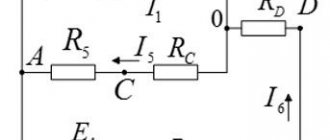
Let us designate the currents in the circuit arbitrarily. Let us denote the directions for traversing the contours. Let's write a system of equations: we will compose three equations according to the first law (one less than the number of nodes) and three equations according to the second law, since there are six unknown currents and the system should consist of six equations.
From simple physical considerations, 1 and 2 Kirgoff rules are derived, which are the basis for calculating currents...
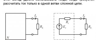
Start of TOE. Method of nodal potentials. An example of solving problems on TOE using the method of nodal potentials is shown....
Since the values of the three currents are unknown, the minimum number of equations to solve the problem is three.
As we remember, Ohm's law relates current, voltage and resistance. If we know any two of these quantities, we can easily find the third. In this case, we know the resistance and the current that flows through that resistance.
In these equations, the EMF value is taken with a “+” sign if the direction of the EMF coincides with the direction of the circuit bypass.
But the more complex the scheme, the more transformations you will have to deal with. For example, first the circuit will need to be reduced to one circuit, the required values must be found, then gradually expanded, producing more and more calculations.
The joint solution of any three equations (1-21a) and equations (1-23) and (1-24) gives the values of currents in all branches of the electrical circuit shown in Fig. 1-18, a.