SIMPLE OSCILLOSCOPE
I. Do lezhelek, M. Munzar (CSFR)
The cathode ray oscilloscope, which will be discussed in the article, is designed to study constant and variable signals with a frequency of 0 ... 5 MHz. Its main advantages are the calibrated sensitivity of the vertical beam deflection amplifier and the sweep duration, which allows not only to observe the signal, but also to measure its parameters, as well as its relatively small size.
Oscilloscope Specifications Vertical Beam Deflection Channel
For convenience of working with the oscilloscope, the numerical values of the deviation coefficients of the vertical deflection channel (VDC) of the beam and the sweep duration are selected as multiples of 1, 2 and 5. It is possible to step-by-step increase the sensitivity of the horizontal deflection channel (VDC) by 10 times (“Temporary Magnifier”), smoothly regulating the level of the signal under study and the duration of the sweep, starting the sweep at any point of the signal's rise or fall.
The functional diagram of the oscilloscope is shown in Fig. 1. The signal under study, supplied to the input jack XW1, is sent through the switch SA100 to the input divider A1, with the help of which it is attenuated to the required level. The divider is designed in such a way that its input resistance remains unchanged for all division ratios. This allows you to connect an external divider between the controlled device and the oscilloscope input, which has little effect on the circuits under study.
The signal under study is amplified by the KVO amplifier A2 and supplied to the corresponding deflecting plates of the cathode ray tube (CRT) VL1, deflecting the beam in the vertical direction; a constant voltage regulated by the variable resistor R103 is supplied to the other input of the amplifier, the level of which determines the vertical position of the oscillogram on the CRT screen. The clock voltage is removed from the output of one of the amplifier stages to internally trigger the time base.
Rectangular pulses with an amplitude of 1 V with a repetition frequency of about 1 kHz, necessary for monitoring the calibration of the CVO and checking the frequency compensation of the remote divider, are generated by generator G1.
For the horizontal deflection beam, either the time base voltage or an external voltage is used if the oscilloscope is operating as an X-Υ indicator.
The time base device includes a ramp voltage generator and a trigger pulse generator. The first of them is made in the form
Miller integrator, controlled by flip-flops DD2 and U1, and can operate in standby and self-oscillating modes. The integrator is formed by an inverting amplifier A4, a feedback capacitor Ct and a charging resistor Rt. A step change in the sweep duration is carried out by switching the RtCt circuits with the “Time/div” switch, a smooth change is carried out by changing the charging current of the integrator with a variable resistor Jft14. The sawtooth voltage is supplied through the isolation amplifier A7 to socket XS3 for use, for example, in a sweep frequency generator.
Pulses from the output of trigger DD2 are amplified by isolation amplifier A6 and, through a high-voltage capacitor (CI0 + C11), are supplied to the CRT modulator VL1 to illuminate the beam. The DC component of the voltage is restored by the diode VD16. Unfortunately, this circuit solution has a significant drawback: due to the presence of a capacitor illumination signal in the circuit, the beam begins to glow after some time even without a sawtooth voltage. However, this drawback only appears in the absence of a synchronizing signal in the standby sweep mode, when a dot on the left side of the CRT begins to light. The authors' experience has shown that this is not dangerous for the used CRT; however, it is not worth leaving it in this state for a long time.
As can be seen from the diagram, the synchronizing voltage at the input of the trigger pulse generator can be supplied through switch SB103 (“Trigger”) or from the KVO amplifier A2 (“Internal”) or from socket XS2 (“External”). The AZ comparator and the Schmitt trigger U2 form triggering pulses from this voltage, the fronts of which are driven by a variable resistor R109 and a switch
SA101 can be placed at any point on the clock signal, i.e., the sweep can be started at any point on the time curve of the signal being studied.
The operating mode of the time base device is selected by switch SB 102. In its “Wait” position, the sawtooth voltage generator operates in standby mode, in the “Auto” position - in self-oscillation mode (pulse detector U3 switches it to this mode).
If the oscilloscope is used as an X-Y indicator, the ramp voltage generator is turned off. Its inverting amplifier in this case acts as a pre-amplifier for the external deflection voltage supplied to socket XS2.
The deflection voltage (sweep or test) is supplied to the input of the A5 KGO amplifier, which amplifies it to the level necessary for deflection by the plates Χι, Xg CRT VLI. Switch SB101 is used to change the gain of amplifier A5 by 10 times, variable resistor R116 is used to shift the beam horizontally.
The oscilloscope uses a B10S3 flat screen CRT. Its power supply is organized in such a way that the voltage on the deflection plates and on the second anode (relative to the common wire) is +100 V, and on the cathode - about -1,160 V. The CRT modulator is connected to the variable resistor R102 (“Brightness”) motor, thanks whereby the voltage on it can be varied from 0 to -40 V (relative to the cathode), which corresponds to complete extinction of the beam.
The oscilloscope's power supply produces stabilized voltages + 5, +12 and -12 V and unstabilized +200 and -I 200 V. Powering the CRT with an unstabilized voltage leads to the fact that when the network voltage fluctuates, the size of the oscillograms changes slightly, but for a simple oscilloscope this can be considered acceptable.
The schematic diagram of the oscilloscope input divider is shown in Fig. 2. Two-stage divider, each stage consists of two frequency-compensated attenuation units with adjustable input capacitance. The first stage links attenuate the signal by 10 and 100 times, the second – by 2 and 5 times. Using the SA100 switch, various combinations of links create nine multiples of 1, 2 and 5 divisor transmission coefficient values from 1 to 0.002.
The amplitude calibrator is made on the DD1 chip. Three of its elements (DDI.1—DD1.3) are used in a rectangular pulse generator, the fourth (DD1.4) is used as an electronic switch that shunts the divider R2R3, from which a calibrated voltage of 1 V is removed. The frequency of the generated oscillations depends on the capacitance of capacitor C2 and the resistance of the resistor RI.
The schematic diagram of the vertical beam deflection amplifier is shown in Fig. 3. Symmetrical three-stage amplifier, the connection between the stages is galvanic. The first stage is assembled according to the source follower circuit on field-effect transistors VT1, VT2 and weakens the influence of the amplifier on the input divider, the second stage (VT3-VT6) performs the functions of an inverter and a broadband amplifier with low output resistance, the third is the final stage
Rice. 3
(VT7, VT8) - amplifies the signal to the amplitude necessary to deflect the beam by the plates and the entire CRT screen. The amplifier gain is adjusted by trimming resistor R16, in the region of lower frequencies it is corrected by resistor R27, in the region of middle frequencies by resistor R28. In the region of higher frequencies the frequency response is determined by the time constant of the circuit R29C4 The quiescent current of the transistors of the final stage is set with trimming resistor R24, the beam in the middle of the screen (with the resistor R103 slider in the middle position) - with trimming resistor R9.
The gain of the amplifier in question is deliberately chosen to be relatively small (the sensitivity of the oscilloscope is only 20 mV per division, whereas usually this parameter is about 10 times better), which is due to the unsatisfactory characteristics of available field-effect transistors, which significantly and, most importantly, inconsistently change their parameters with temperature fluctuations.
The trigger pulse generator (Fig. 4) includes a comparator on transistors VT1—VT3, a Schmitt trigger on elements DD1.1, DD1.2, a polarity switch on elements DD1.3, DD1.4, DD2.1—DD2.4 and device for automatically starting a sawtooth voltage generator using transistor VT4 and elements DD3.1, DD3.2.
The internal or external (from socket XS2) synchronizing signal is limited in the comparator to a level depending on the voltage (within - 5 ... + 5 V) removed from the variable resistor R109. From the output signal of the comparator, the Schmitt trigger generates square oscillations with the levels necessary for the operation of subsequent devices based on TTL elements. The desired polarity of trigger pulses is selected using switch SA102.
The output pulses of element DD2.2 are inverted by inverters DD2.3 and DD2.4 and are supplied from the first of them to the input of the pulse detector (VD1, VD2, VT4), and from the second to the differentiating circuit C5R11. The narrow trigger pulses generated by it, corresponding in time to the rise or fall of the synchronizing signal (depending on the position of the SAI02 switch), are supplied to one of the inputs of the DD3.2 element. Its other input is connected to the output of the pulse detector. In the presence of a synchronizing signal, element DD3.2, regardless of the position of switch SB 102, generates narrow trigger pulses, which are supplied to coincidence element DD4.1 of the sawtooth voltage generator trigger. If there is no synchronizing signal, then in the “Auto” mode, the output of the DD3.2 element is constantly present with a voltage of logical 1, and in the “Standby” mode - logical 0.
The Miller integrator, which generates a sawtooth sweep voltage, is formed by an inverting amplifier on transistors VT6, VT7, a set of integrating capacitors Ctl - Ct6 and charging resistors R110 - R113. The operation of the integrator is controlled by an RS trigger on elements DD4.2, DD4.3 and a Schmitt trigger on transistor VT5 and elements DD3.3 and DD4.4.
In the initial state (beam on the left side of the CRT screen), the voltage level at the output of the RS flip-flop (pin 8 of element DD4.3) corresponds to logical 1. For this reason, the diodes VD4 and VD100 are open, the capacitor connected to the integrator is short-circuited, and the output voltage device is equal to 0. With the arrival of the trigger pulse, the RS trigger changes its state, the high voltage level at its output is replaced by a low one, and the voltage at the integrator output begins to increase. The steepness of its increase depends on the capacitance of the capacitor Ct, the resistance of the resistor Rt (R110—R112) and the position of the variable resistor R114,
At the same time, one of the capacitors Ch begins to charge through the diode VD7. When the voltage reaches a given level, the Schmitt trigger is triggered and the RS trigger returns to its original state. As a result, diodes VD4, VD100 open again, and the charged capacitor Ct is quickly discharged. At the same time, but somewhat more slowly, capacitor Ch is discharged through resistors R15, R16. And until the voltage across it decreases to a certain level, neither the Schmitt trigger nor the RS trigger changes its state, so no triggering pulse can disrupt the normal operation of the generator. The formation of the next cycle of voltage increase begins either with the arrival of the next triggering pulse, or (in the absence of pulses in the “Auto” mode) immediately after the RS trigger transitions to the single state (low level at the output of element DD4.3).
The sweep duration is changed by switching capacitors Cti-Ct, Chi-Ch6 and resistors R110-R112.
The sawtooth voltage is supplied to the output jack XS3 through an emitter follower on transistor VT8.
When using an inverting amplifier to amplify the deflection signal, the gain is determined by the resistance of resistor R107. The R105R106 divider creates the bias voltage needed to center the beam on the CRT screen.
The amplification stage on transistor VT12 amplifies the output pulses
RS trigger up to an amplitude of 30 V. Diode VD3 protects the transistor from breakdown when the voltage increases - 1,200 V.
The KGO amplifier consists of a pre-amplification stage on transistor VT9 and a symmetrical output stage on transistors VT10, VT11. The quiescent current of these transistors is set by trimming resistor R39, the sensitivity of the amplifier as a whole is set by resistor R28, and an increase in gain of exactly 10 times when the contacts of switch SB101 is opened is achieved by resistor R33. Variable resistor R116 is used to move the oscillogram horizontally. Diodes VD5, VD6 prevent transistor VT10 from saturating, thus reducing the delay of the sweep signal by the amplifier.
The schematic diagram of the oscilloscope power supply and CRT circuits is shown in Fig. 5. Voltages +5, +12 and -12 V are created by rectifying the alternating voltage of windings II and III of network transformer T1 with a diode bridge VD1-VD4. Capacitors Cl, C2 reduce interference to broadcast reception in the form of a multiplicative background that occurs when switching diodes during voltage rectification. In order to reduce output voltage ripple, U-shaped RC filters C5R1C7, C6R4C8 and C5R7C9 are included in the power supply circuit of the zener diodes VD9, VD10, VD15.
The same filters are also used in sources of unstabilized voltages of +200 and -1200 V. Resistors Rl 1 and R12, R13 and RI4, R16-R18 equalize the voltages applied to the series-connected oxide capacitor frames C11 and C12, C13 and C14, C15 —C17. Capacitors SZ, C4 perform the same functions as capacitors Cl, C2.
The brightness of the image on the CRT screen is adjusted with variable resistor R102, the beam is focused with variable resistor R101, and the most round shape of the luminous spot is achieved with trimming resistor R10.
Trimmer capacitor G100 compensates for the mutual parasitic capacitance of the horizontal and vertical deflection plates of the CRT.
LED VD101—indicator that the oscilloscope is connected to the network.
The output resistance and capacitance of the oscilloscope, independent of the position of the input divider switch, allows you to connect an external divider between it and the controlled circuit. Typically, the division ratio of such devices is 1:10. The increased input resistance of the divider (10 MΩ) with a relatively small input capacitance (about 15 pF) makes it possible to study high-frequency and pulse circuits that are sensitive to external influences.
The schematic diagram of a simple 1:10 remote divider for the described oscilloscope (R„=l MΩ, Cax=35 pF) is shown in Fig. 6. The input voltage divider is formed from a series circuit of resistors R1-R3 and the input resistance of the oscilloscope, shunted respectively by the capacitor CI and the input capacitance of the device. By changing the capacitance of capacitor C1, it is possible to ensure that the attenuation introduced by the divider will be practically independent of frequency over the entire operating range.
A possible design option for an external divider is shown in Fig. 7. Its body consists of brass front (4) and rear (9) rings and covers 8 soldered to them, bent in the form of grooves made of tinned sheet metal 0.3 mm thick. Case diameter -15, length -80 mm. After assembly, a polyvinyl chloride sheet is stretched over it
Rice. 5
tube of suitable diameter. Using an insulating sleeve 5 (fiberglass plastic) a crocodile clip is fixed in the front ring, and a coaxial cable 10 with a characteristic impedance of 75 Ohms, ending with a coaxial connector plug, is fixed in the rear ring using a rubber ring. In order for the capacitance of capacitor 1 (C1) to be as small as possible, the distributed capacitance of the cable should be as small as possible, and the length should be no more than 1 m. The cable braid and the flexible common wire ending with plug 2 are soldered to the bottom (as per Fig. 7) cover at one point.
Resistors 6 (R1 - R3) on one side are soldered to terminal 3, on the other - to the terminal of trimmer capacitor 1 (C1) glued to cover 8. The total resistance of the resistors should not exceed 9 MOhm ± 2%. Trimmer capacitor C1 is ceramic.
The most structurally complex oscilloscope unit is the input divider (see Fig. 2), since it unfavorably manifests parasitic capacitance between the parts of the links: it causes the appearance of emissions in the square oscillations under study, which cannot be eliminated by compensating capacitors. Therefore, the design of the divider and, in particular, the switch used in it, must first of all provide sufficiently good shielding of circuits critical to the formation of parasitic connections.
To switch the links, the authors used a modified biscuit switch WK 533 44 (domestic switches PG2-4 have a similar design. - Ed.). The modification consists of installing a shielding partition, removing excess moving contacts from the first two sections and introducing additional contacts into the rest so as to obtain the switching circuit shown in Fig. 2. This is how it is done. The switch is disassembled, the shielding partition (Fig. 8, a), made of tinned sheet metal 0.3 mm thick, is installed in place of the plastic ring of the third section equipped with internal teeth. The rotor of this section is removed. Movable contacts I (Fig. 8, b), introduced in addition to contacts 3, are inserted together with springs into holes drilled in rotors 4 of the fourth and fifth sections. To avoid short circuits between the springs of contacts 1 and the metal knife of the switch, pieces of nylon fishing line 2 with a diameter of 0.8 mm are placed between them, for which recesses of the same depth are cut out in the knife.
Rice. 8
During assembly, ensure alignment of the knife and the switch roller, after which they are connected by soldering. The threaded rods that secure the switch sections to its body are soldered to the metal back wall, which is “grounded.”
The input divider housing (Fig. 9) consists of a U-shaped base 1 and a cover 7, bent from 0.6 mm thick tinned sheet metal. They are connected to each other with M2.5X5 screws screwed into threaded posts 5. Switch 3 is fixed to the base with a nut, their rear walls are connected to one another with a short wire. Shielding partition 2 is soldered to the base and foil of the common wire of printed circuit board 6 (Fig. 10; a - drawing of the board, 6 - arrangement of elements on it), made of foiled fiberglass laminate 1.5 mm thick. It is secured to the base shelves with the same screws as the threaded stands 5. To fasten the divider to the front wall of the oscilloscope, use two nuts 4 (M2), soldered to the front wall of the base from the rear side.
Trimmer capacitors C2, SZ, C5, C6, etc. are ceramic with a diameter of 8 or 10 mm (you can use any other ceramic capacitors, it is only important that they fit in the places allocated for them on the printed circuit board. - (Note, ed. ).
The permissible deviation of the resistances of resistors R1—R8 from the values indicated on the diagram should not exceed ± 1%. If it is impossible to select resistors with such accuracy from the available specimens, it is recommended to adjust (using, for example, a digital ohmmeter) the resistance of metallized resistors of the nearest lower values. To do this from a resistor
Carefully remove the protective varnish, connect its leads to an ohmmeter and, using a hard school eraser, carefully erase the conductive layer until the resistance is within the specified limits. All that remains is to cover this layer with a protective varnish, and the desired resistor is ready.
In the same way, you can adjust the resistances of resistors R2, R3 of the amplitude calibrator, R1 of the KVO amplifier and R110-R112 of the time base device (they also should not differ from those indicated in the diagram by more than ± 1%). Capacitors, Ctl-Ct6, Chl-Ch6, should also be selected with almost the same accuracy (A...2%).
Capacitors C12 of the input divider, Cl-C5 of the KVO amplifier, C1, C2, C4, C12, C13, Ctl, Chl of the time base device, Cl, C2 of the power supply - ceramic, C4, C7 of the input divider and CJ, Cl 1 in the CRT modulator circuit — polystyrene. Variable resistors R101—R103, R109, R114, R116—group A.
It should be noted that on each of the equalizing resistors R11—R14, R16—R18 the voltage drops more than 200 V, so you cannot use small-sized resistors.
In the sweep device, you can use a switch for a smaller number of positions, for example twelve. In this case, the sweep duration values need to be recalculated into multiples of 1, 3, 16, 10 and expand the range of smooth adjustment with variable resistor R114, reducing the resistance of resistor R113.
Most of the oscilloscope parts are mounted on printed circuit boards made of foil fiberglass. A drawing of the board and the location of the amplitude calibrator parts on it are shown in Fig. 11, KVO amplifier - in Fig. 12, boost-
Rice. 12
Rice. 13
Rice. 14
Rice. 15
For KGO and time base nodes - in Fig. 13. The power supply is located on two printed circuit boards: on one of them (Fig. 14) voltage sources + 5, +12, -12 and +200 V are mounted, on the other (Fig. 15) voltage sources +1,200 V are mounted.
Transistors VT1, VT2 of the KVO amplifier and regulating transistors VT1 - VT3 of the power supply voltage stabilizers are connected using sockets. In the first case, this is due to the need to select field-effect transistors in an already assembled oscilloscope, in the second, due to the possible failure of transistors during setup, since to simplify the power supply, the authors refused to introduce devices for protecting stabilizers from overloads. All digital integrated circuits are connected using the panels.
The power transformer T1 is wound on a magnetic core ΕΙ32Χ25 from oriented permalloy plates with a thickness of 0.105 mm. Winding I contains 1200 turns of wire PEV-1 0.28, windings II, III and IV - 80, 80 and 1200 turns of wire PEV-1 0.2, respectively, winding V - 2550 turns PEV-1 0.1, winding VI— 25 turns PEV-1 0.67. The electrostatic screen between the network and other windings is 1.5 turns of copper foil, wrapped in varnished cloth 0.2 mm thick. Three layers of the same varnished fabric are laid between windings IV and V, and one layer between the others. Interlayer insulation in the windings is transformer paper 0.05 mm thick.
For better cooling, resistors R30, R31 of the KVO amplifier and R43, R44 of the KGO amplifier are installed at a distance of 8 mm from the printed circuit boards, and transistors Vi? ut8 perV0G0 of them and VT10, VT11 of the second are equipped with heat sinks bent from duralumin or brass, as shown in Fig. 16. The gaps between the transistor housings and heat sinks are filled with silicone grease.
The appearance of the oscilloscope is shown in Fig. 17, the structure of its body and the placement of parts in it are shown in Fig. 18. The body consists of duralumin front (12) and rear (4) panels, screwed with screws 3 (M4X 10) to four ties 2 of the same material. Wall 1 is also attached to them, and to it and the front panel 12 is a partition 16 (both made of solid aluminum alloy), dividing the lower part of the oscilloscope into three shielded compartments. Drawings of the front and rear panels of the device are shown in Fig. 1, respectively. 19 and 20, couplers 2—in Fig. 21, walls 1 and partitions 16—respectively in Fig. 22 and 23.
The finished front panel of the oscilloscope case is sanded with fine-grained sandpaper, etched in alkali and painted with matte black paint. Inscriptions explaining the purpose of the controls and connections are made in a transferable font (white on black and black on white).
Rice. 19
The bottom and upper U-shaped cover are made of solid aluminum alloy with a thickness of 1.5 mm. To cool the heating parts of the oscilloscope, ventilation holes are drilled in the bottom, and to ensure that there is always sufficient distance between it and the table plane, rubber feet of the appropriate height are screwed on. The cover is covered with artificial leather and equipped with a handle for carrying the oscilloscope. A ventilation hole measuring 100 X 60 mm is cut under the handle, covered with a metal mesh. The bottom and cover are screwed with MZH5 screws to the lower ties of the housing.
Rice. 20
Rice. 22
Rice. 23
The cathode ray tube is placed in a casing 9, spot welded from permalloy 0.5 mm thick, followed by heat treatment. A felt ring is glued into the front (according to Fig. 18—right) part of the casing, into which the part of the CRT bulb adjacent to the screen is inserted. The plastic base of the CRT is held in place by a steel clamp soldered into the back of the casing and covered with thin felt.
The casing with the CRT is inserted into the oscilloscope housing from above. At the front it is placed on a bracket 13, bent from a steel tape 0.5 mm thick and screwed to the upper ties, at the back, on the wall 1. The casing is pressed to the bracket with a spring made of steel wire, to the wall - with a leather belt 11, screwed to the both sides with threaded duralumin nuts 10. The hole in the rear panel for the CRT base is covered with a plastic cover, the window for its screen in the front panel is covered with a plate of transparent organic glass 3 mm thick. From the inside, using self-adhesive tape, a positive with a raster shown in Fig. is glued to the plate. 24, covered with a green-blue transparent film that increases the contrast of the image. Above the screen in the front panel there are two M3 threaded holes for screws for hanging a tube that protects the screen from unwanted side light.
Under the CRT casing, to the left of the partition 16 (if you look at the oscilloscope from the front), there is an input divider 15, a KVO amplifier and an amplitude calibrator 14, on the right is a time base device with a KGO amplifier. The protrusions of the printed circuit boards of the KVO amplifier and the time base device with the KGO amplifier are inserted into special U-shaped holders mounted on the partition and can be rotated at an angle of about 90°. In the working position, the boards are screwed to threaded posts, which are also fixed to the partition. The distance between the latter and the KVO amplifier board is 11, between it and the scanner board is 43 mm (filter capacitors C101, C102 are installed here).
In the lower part of the rear compartment of the case there is a power transformer 5, above it there are U-shaped plastic guides 7, into which printed circuit boards of the power supply 6 and 8 are pushed. Above them, in the holes of the wall 1, variable resistors R101, R102 (their bushings) are fixed and the nuts are insulated from it) and a push-button power switch, and in the holes in the rear panel 4 there is a fuse holder and a power cord.
The power switch is connected to the button on the front panel by a rod made of a metal rod with a diameter of 4 mm. The textolite rollers extending the axes of variable resistors R101, R102 also have the same diameter.
The VD101 LED with resistor RU7 is mounted on a miniature (15X 10 mm) printed circuit board secured to the front panel 12 using a screw and a threaded stand.
Variable resistors R103, R108, R114, R116 are fixed with their nuts directly on the front panel, the input divider and sweep duration switch are screwed to it with M2X6 countersunk screws. The handles of the last two controls are equipped with dials (Fig. 25), made using a photo method.
Push-button switch SB101—SB104 with independent fixation of buttons is attached to the front panel using screws and threaded stands, switch SA102 (miniature toggle switch) is glued into a duralumin prism screwed to the panel at the back, switch SA100 (toggle switch with three positions) is fixed using a bracket (with If possible, it is advisable to replace it with a slide switch). Coaxial jack XW1 is ENC brand with a characteristic impedance of 50 Ohms.
To select parts and set up an oscilloscope, an RLC bridge, a pulse generator (the simplest device on TTL chips will do) and a voltmeter with a high input impedance are enough. Naturally, having a good oscilloscope, digital multimeter and digital capacitance meter will speed up the work significantly.
Setup begins by checking the power source. If the parts are in good condition and there are no installation errors, all output voltages should not differ from those indicated in the diagram by more than ± 10%. Having verified this, they check the functionality of the time base, the KVO and KGO amplifiers, the input divider and the amplitude calibrator.
Adjusting the time base device comes down to setting (with trimming resistor R15) the sawtooth voltage swing equal to 8 V. If you don’t have an oscilloscope, you can limit yourself to an approximate estimate of the swing by measuring with a voltmeter with a high input impedance voltage at the collector of the VT7 transistor at the maximum sweep duration.
To adjust the KGO amplifier, switches SA101 and SB10I are set to the “1 ms” and “XI” positions, respectively, move the variable resistor R114 to the upper (according to Fig. 4) position and, applying an alternating voltage of a reference frequency of 1 kHz to the input jack XW1, use a trimming resistor R28 ensure that the oscillation period occupies exactly five divisions in the middle of the CRT screen. Then switch SB101 is moved to position “X 10”, the frequency of the measuring signal is increased to 10 kHz and the same result is achieved with trimming resistor R33.
The quiescent current of the transistors of the final stage of the KGO amplifier is set with a trimming resistor R39, trying to ensure that the scan line on the CRT screen becomes as long as possible and does not expand at the edges.
In conclusion, it is necessary to ensure that when the contacts of the SB101 button are opened (transferring it from the “X 1” position to the “X 10” position), the midpoint of the scan line remains in place. In the position of the “XI” button, it is shifted to the center of the screen with a trimming resistor R37, in the “XY” position - with a variable resistor R116. If necessary, these operations are repeated several times. This also applies to all other adjustments: due to the direct (galvanic) connection between the adjustment nodes, they can mutually influence each other, so all the operations described above must also be repeated several times.
Setting up a KVO amplifier begins with the selection of field-effect transistors of the first stage. To operate in an amplifier, first select specimens with a voltage in the range of 0...3 V (measured between the source of the transistor and the common wire), and from them - two such ones for which this voltage is approximately the same (a difference of no more than 0.5 V is allowed). After this, the temperature drift is determined - the displacement of the beam (or rather, defocused - to avoid burning through the phosphor - spot) for 30 minutes, counting from the moment the oscilloscope is turned on. A beam displacement of less than 10 mm can be considered acceptable.
Next, the amplifier board is installed in place, the SA100 switch and the variable resistor R103 slider are moved to the middle position and the trimming resistor R9 is used to move the beam to the middle of the CRT screen. Then, using trimming resistor R24, a voltage of 100 V is set on the collectors of transistors VT7, VT8 and proceed to adjusting the frequency response. To do this, switches SA100 and SAI of the input divider are moved respectively to the “~” and “20 mV/div” positions, rectangular pulses with a repetition frequency of 0.1 ... 1 MHz are supplied to the input jack XW1 and by alternately turning the sliders of resistors R27 and R28, undistorted images of pulses on the screen (without emissions and with possibly steeper front and fall).
The adjustment of the KVO amplifier is completed with calibration, but first the output voltage of the amplitude calibrator itself is calibrated. To do this, connect a voltmeter with a relative input resistance of at least 20 kOhm/V to the output of the calibrator and determine the difference in its readings when a voltage of -|-5 V is applied to the inputs of element DD1.1 and connected to the common wire. If this difference is not exactly 1 V, select the resistance of one of the resistors R2, R3. This is best done by shunting it with a resistor of higher resistance.
Then the output of the calibrator is connected to socket XW1, the input divider is set to the “200 mV/div” position. and the tuning resistor R16 ensure that the amplitude of the rectangular pulses on the CRT screen becomes equal to exactly five divisions.
The last thing to adjust is the input divider. By setting its switch to the “50 mV/div” position, rectangular pulses with a repetition frequency of 1 kHz are supplied to the input and the capacitance of the tuning capacitor C8 is selected at which the rises and falls of the pulses are least distorted. Then the same result is achieved by sequentially moving the switch to the “100 mV/div” position. (capacitor SJ), “0.2 V/div.” (C2) and “2 V/div.” (C5).
Next, the input capacitance of the oscilloscope is equalized. The easiest way to do this is to directly measure it with a capacitance meter. The task in this case comes down to measuring the input capacitance at the “20 mV/div” position. and then setting the same value in the “50 mV/div” positions. (tuning capacitor C9), “100 mV/div.> (SP), “0.2 V/div.” (NW) and “2 V/div.” (C6). It should be noted that only a device with a voltage of no more than a few volts applied to the capacitance being measured is suitable for these measurements. If there is no such device, then by setting the input divider switch to the “20 mV/div” position, rectangular pulses are supplied from the generator to the oscilloscope input through an external 1:10 divider. Having achieved minimal distortion of the edges and decays of pulses on the CRT screen using the trimmer capacitor of the remote divider, sequentially switch the input divider to the positions “50 mV/div,” “100 mV/div.”, “0.2 V/div.”, “2 V/div.” business." and the same goal is achieved with tuning capacitors C9, Cl 1, SZ and C6. The pulse repetition rate is selected such that distortions in their shape are clearly visible before adjustment.
Finally, the CRT beam is as round as possible and the mutual capacitance of the horizontal and vertical beam deflection plates is compensated. The first of these adjustments is made by trimming resistor R10 of the power supply with the beam slightly defocused (in order to increase the diameter of the luminous spot). Then a square voltage with a frequency of 1 MHz is applied to the input of the oscilloscope and the scan is turned on by pressing the SB 104 button. In an ideal case, that is, in the absence of parasitic capacitance between the above plates, a segment of a straight vertical line should be observed on the CRT screen. However, since such a capacitance exists, instead of a straight line on the screen, a certain figure resembling the number 8 is usually observed. The task is to reduce the area of this figure as much as possible with the tuning capacitor C100.
When working with an oscilloscope, it is necessary to remember that the sensitivity in volts per division, set by switch SA1, corresponds to the true one (of course, taking into account the error) only when the signal under study is applied directly to its input. If the signal comes through an external divider, the sensitivity value set by the switch must be multiplied by 10.
The sweep duration set using the switch SA101 corresponds to the true one only when the slider of the variable resistor R114 (“Sweep duration smoothly”) is in the uppermost position (according to the diagram shown in Fig. 4), and the SB101 switch is in the lower one (also according to the diagram) provisions. By moving the slider of resistor R114 in the opposite direction, the sweep duration can be reduced by about 3 times.
It should also be remembered that the use of a “time magnifying glass” (SB101) is limited by the low brightness of the beam in this operating mode, and due to the insufficiently wide bandwidth of the KGO amplifier, its use with a sweep duration of less than 1...2 μs per division (practically in the first two switch SA101) is not possible.
Source: Designs of Soviet and Czechoslovak radio amateurs: Sat. articles/Composition: A. V. Gorokhovsky, V. V. Frolov—Book. 4.— M.: Radio and Communications, 1991.— 208 p.: ill.— (Mass Radio Library. Issue 1169).
Tweet Like
- Previous post: NON-CONTACT CAPACITIVE SENSOR – DO IT YOURSELF
- Next entry: Hardware COM-IR interface module
- What is the difference between current and voltage? (2)
- Current and Voltage Relationship (0)
- AUDIO PREAMPLIFIER WITH AGC (2)
- POWER SUPPLY FOR CAR RADIO (0)
- BATTERY CHARGER (0)
- LITHIUM-NON CELL CHARGER CHARGER CONTROLLER (0)
- BATTERY CHARGING CURRENT LIMITER (0)
Related posts:
Measurement technique
The oscilloscope measures electrical voltage and generates an amplitude graph of electrical fluctuations. Digital devices can remember the resulting schedule and return to it.
Oscillations are displayed on the screen in a two-dimensional coordinate system (voltage is the vertical axis, time is the horizontal axis), forming a graph - an oscillogram. There is a third component of research - signal intensity (or brightness).
If there are no input pulses on the screen, the horizontal line is “zero”, indicating the absence of voltage. As soon as voltage is applied to the input (or inputs) of the device, one or several graphs become visible on the screen simultaneously (depending on the number of measured signals).
The shape of a graph of electrical vibrations can be:
- sinusoid;
- damped sinusoid;
- rectangle;
- meander;
- triangles;
- sawtooth vibrations;
- pulse;
- difference;
- complex signal.
To obtain a stable graph of oscillations, the device contains a synchronization unit. It is possible to obtain a cyclic display of oscillations only after setting the synchronization value. It is taken as the “starting” one and serves as the starting point of the schedule. All jumps are displayed relative to this point.
How to choose
You need to imagine for what purposes and how often the device will be used, to study what signals it is intended for. Consider the number of points for simultaneous measurement, singleness or periodicity of oscillations. Sometimes Soviet-made devices are used. But getting precise tuning with them is difficult.
Number of channels
By the number of channels, oscilloscopes can be single-channel, simple (2-4 channels), advanced (up to 16 channels). Multiple channels allow you to simultaneously analyze incoming signals.
2.3. Addition mode.
The algebraic sum of the signals CH1 (Channel 1) and CH2 (Channel 2) can be observed on the screen by setting the VERT MODE switch to the ADD position, the difference of the signals if the CH2 INV switch is pressed (CH1-CH2).
For more accurate calculations, it is desirable that the sensitivity of each of the two channels be the same, which can be done using the VARIABLE buttons. Vertical movement can be made with the VERTICAL POSITION knob of any channel. Due to the linearity of vertical amplifiers, place both buttons in their middle positions.
2.1. Single channel mode.
Before turning on the instrument, ensure that the ground terminal is connected to ground and the oscilloscope controls are set to the positions shown below:
| Name | Number | Switch position |
| POWER | (6) | Pressed out |
| INTEN | (2) | Middle position |
| FOCUS | (3) | Middle position |
| VERT MODE | (14) | CH1 |
| ALT/CHOP | (12) | Pressed (ALT) |
| CH2 INV | (16) | Pressed out |
| POSITION | (11)(19) | Middle position |
| VOLTS/DIV | (7)(22) | 0.5V/div |
| VARIABLE | (9)(21) | CAL (far right position, clockwise) |
| AC-DC-GND | ( | GND |
| SOURCE | (23) | CH 1 |
| SLOPE | (26) | + |
| TRIG ALT | (27) | Pressed out |
| TRIGGER MODE | (25) | AUTO |
| TIME/DIV | (18) | 0.5ms/div |
| SWP. VAR | (30) | Far right position |
| POSITION | (32) | Middle position |
| X1O MAG | (31) | Pressed out |
| LEVEL | (28) | Middle position |
After installing the controls as above, plug the power cord into the wall outlet, and then continue as follows:
1) Turn on the NETWORK button and make sure the network indicator lights up. Within approximately 20 seconds, a scan line should appear on the screen. If the beam does not appear within approximately 60 seconds, check that the controls are installed correctly.
2) Set the desired brightness and focus of the image using the BRIGHTNESS and FOCUS knobs.
3) Apply a signal to the CH1 (Channel 1) input
4) Set the AC-DC-GND switch to AC position. The signal image should be visible on the screen.
5) Adjust image clarity using the FOCUS knob
6) Use the VOLTS/DIV and TIME/DIV switches to set the desired signal sizes.
7) Using the switches, align the signal image with the scale lines so that you can easily calculate the amplitude (Vp-p) and period (T).
The above is the basic principles of working with an oscilloscope when channel 1 (CH 1) is turned on. When working with channel 2, do the same.
Formation of signals of triangular, rectangular and sinusoidal shapes
1. First select the output waveform (8), range (7); By rotating the FREQUENCY knob (13), adjust the desired frequency (its value will be indicated on the display).
2. Connect output (22) to an oscilloscope or other device to observe the output waveform.
3. Rotate the AMPL knob (12) to set the required signal amplitude.
4. If signal attenuation is required, pull out the AMPL control (12) to obtain 20dB of attenuation, or press the control (12a) for an additional 20dB of attenuation.
5. Types of output signal shapes and phase relationships are shown in Fig. 4:
Rice. 4 Fig. 5
2.2. Dual-channel operating mode.
Set the VERT MODE switch to the DUAL position. On the screen, in addition to the signal from channel 1, a straight line of channel 2 will be observed (the controls must be set as described above).
Apply a signal to the second channel. Set the AC-DC-GND switch to the AC position. Set the image using the V/DIV and TIME/DIV knobs.
When using dual channel mode (DUAL or ADD mode), the signal of channel 1 or channel 2 can be synchronized by toggling the SOURCE switch. If both CH1 (Channel 1) and CH2 (Channel 2) signals are equivalent, then they can be stably displayed simultaneously;
If not, only the channel signal selected by the SOURCE switch can be displayed permanently. If you press the TRIG. ALT, then stable observation of two signals is possible. (Do not use "CHOP" and "ALT" switch at the same time). Switching between CHOP mode and ALT mode occurs automatically by changing the position of the TIME/DIV switch.
2.4. Synchronization.
Selecting a trigger is essential for effective operation of the oscilloscope. The user must be fully familiar with the functions of the mode switches and clock sources.
(1) MODE switch purpose:
AUTO (automatic)
Selecting the automatic scanning mode is carried out by setting the switch to the AUTO position. The scan generator operates in self-oscillating mode without a synchronization signal. As soon as the synchronization signal appears, the sweep generator will operate synchronously with the input signal. The AUTO mode is convenient to use when turning on the device to observe the beam and input signal and then turning on other operating modes of the device. Once the controls are set to the required positions, you can return to NORM mode. The AUTO mode should be used when studying constant voltages and signals with small amplitudes when there is no sweep synchronization.
NORM (standby)
The sweep generator will not start until the required sweep trigger level is set with the “LEVEL” knob. The sweep generator generates only one beam path and is subsequently activated only when another synchronization signal is received. In NORM mode, the screen will not display the beam until synchronization occurs. In channel 1 and channel 2 summation mode and NORM sync mode, no channel will be displayed until there is a sync.
modes are not used in laboratory work.
(2) SOURCE switch functions:
The SOURCE switch is used to select the clock source.
CH 1: CH1 amplifier signal, which is used as the clock signal most often.
CH 2: The CH2 amplifier signal is used as the clock signal.
LINE: The AC mains frequency signal is used as the synchronization signal. This method is effective when the measured signal has a time relationship with the network frequency.
EXT. The sweep is triggered by an external signal, which is fed to an external input. Since the sweep is synchronized by the same signal, this allows you to study signals of different amplitudes, frequencies and shapes without rearranging the synchronization adjustments.
(3) Trigger level and polarity selection:
The sweep is started when a certain level is set with the corresponding 'LEVEL' trigger knob. Rotating the knob changes the starting point of the sweep generator. When the knob is rotated to the “+” area, the launch will occur with a positive half-wave; when the knob is rotated to the “-” area, the launch will occur with a negative half-wave; when the knob is in the central position, the sweep will be launched from the zero line.
Rotate the TRIG LEVEL knob to set the desired trigger level. When examining a sinusoidal signal, the initial phase can be changed. Rotating the TRIG LEVEL knob allows you to synchronize the signal from peak to peak.
When the TRIG SLOPE switch is in the “+” position, the sweep is triggered by the positive portion of the clock signal.
When the TRIG SLOPE switch is in the - position, the sweep is triggered by the negative portion of the clock signal. The choice of signal polarity is shown in Fig.
(4) Synchronization with the sum signal (TRIG ALT button):
The TRIG ALT button is used to select different clock sources in dual channel mode (selected by the VERT MODE switch). In this mode, the sweep is triggered alternately by a signal from channel 1 or channel 2. This is necessary when studying signals with different frequencies or periods. In this mode, both signals are synchronized and the image on the oscilloscope screen is motionless. This mode cannot be used when measuring the phase difference between channel 1 and channel 2 signals.
2.6. Signal stretching.
Use the X10 MAG button to view small parts of the signal, such as those located far from the start of the sweep, to examine them using the TIME/DIV knob. To enable MAG mode, follow these steps.
1. Set the TIME/DIV knob to the largest sweep factor that allows you to study this part of the signal.
2. Rotate the HORIZONTAL POSITION knob to position the signal so that that portion of the signal is in the center of the screen.
3. Press the x10 MAG button until the indicator turns on. When performing the above procedures, the required part of the signal will be magnified 10 times to the right.
(Sweep in position in/div ´ 1/10)
Thus, the unstretched maximum sweep speed (0.1 µs/div) can be increased as follows:
0.1 µsec/div ´ 1/10=10 nsec/div
When the sweep is increased and the sweep speed is more than 0.1 µs/div, the brightness of the beam may decrease.
Square wave generation
1. Press the key (P) of the waveform selection field (8); then select the frequency range (7) and rotate the FREQUENCY knob (13) to set the desired frequency.
2. Connect the output jack (22) to an oscilloscope to observe the output waveform.
3. Pull out and rotate the DUTY knob (9) to set the duty cycle of the pulse signal.
4. Rotate the AMPL knob (12) to set the pulse amplitude.
5. Pull out the AMPL control (12) to achieve a 20dB output attenuation.