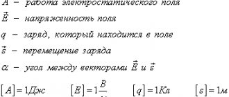
1. Ball on a spring, Newtonian version 2. Quantum ball on a spring 3. Waves, classical view 4. Waves, classical equation of motion 5. Quantum waves 6. Fields 7. Particles are quanta 8. How particles interact with fields Actually We already entered the fields some time ago, I just didn’t warn you about it - I wanted to concentrate on the waves that arise in these fields. In describing how waves behave, we expressed their shape and time dependence using the function Z(x,t). Well, Z(x,t) is a field. It is a function of space and time with an equation of motion that determines its behavior. A suitable motion function would be such that if Z increases or decreases at a certain point, then Z will decrease or increase at neighboring points a little later. This feature allows waves to be among the solutions to the equation.
In this article we will look at some examples of Z(x,t) fields whose equations of motion allow the presence of waves. The physical interpretation of these fields will be very different. They describe different properties of different materials. But the equations they satisfy and the waves they exhibit will satisfy very similar mathematics, and they will behave similarly, despite their different physical origins. This will become a very important point in the future. And then we'll do something radical—look at fields in the context of special relativity. As Einstein showed, if you tweak space and time and make them behave differently than most people expect, you get a new type of field—one whose physical interpretation is not a property of anything else, but a physical object in its own right.
Scalar field
For example, we can measure the temperature in winter at different points in the room.
At the same time, the closer to the central heating radiator and the higher to the ceiling, the higher the temperature will be. And at points near the floor and away from the heated battery, the temperature will be several degrees lower.
Let's consider three-dimensional space (Fig. 1) and some point located in this space. Let's denote the point with a capital letter, for example P.
Rice. 1. Each point in three-dimensional space is associated with three numbers on the axes
This point is associated with three numbers x, y, z, lying on the axes Ox, Oy, Oz. Such numbers are called point coordinates. Mathematicians usually write down the coordinates of a point next to its name: \(\large P\left( x ; y ; z \right)\).
We can additionally assign a fourth number to this point - temperature t in degrees Celsius (Fig. 2).
Rice. 2. Example of temperature distribution in a room during the heating season
Let's compile a table that will contain the coordinates of points in space and the temperature at these points. This way we will organize information about the temperature distribution in the room.
Using such a table, we can construct graphs on which we will depict exactly how the temperature will depend on any spatial coordinate.
This table and graphs contain information about the temperature field.
Since the temperature distributed throughout the room is a scalar quantity, the temperature field is called scalar. And the table specifies a scalar function that describes the temperature distribution in the room.
This function connects the coordinates of a point and the value of a physical quantity - temperature at this point.
This is a common function, like those with which you had to solve examples in school mathematics. Only this function depends not on one variable x, but on three variable quantities - the coordinates x, y, z of points located in three-dimensional space.
\[\large \varphi = f \left( x ; y ; z \right)\]
And the fourth value, temperature, will be the value of this function. Like the number “y” for a function of one variable “x”.
Vector field
Suppose there is a large magnet in the corner of the room. And we walk around the room with a cord, to one end of which an iron nail is tied. We hold the second end of the lace in a horizontally extended hand.
Walking around the room, we will notice that in some area of the room the cord with a nail deviates from its vertical position towards the magnet.
The closer we get to the magnet, the more it attracts the nail. The more effort you need to make to hold the lace in your hand.
Such fields, like the field created by a magnet, are called force fields.
Force fields are vector fields, since the force distributed throughout the room and measured at various points in the room is a vector quantity.
Now we can assign to each point of the room not only the coordinates of the point, but also the vector F of the force acting on the nail at this point.
Let's make a table and write down in it the coordinates of each selected point in the room and the coordinates of the force vector with which the magnet acts on the nail at this point.
The force vector at each individual point will have its own characteristics - length and direction. Therefore, a table containing information about the force at each point in the room will contain 6 rows. Three lines are the coordinates of the point, and three lines are the coordinates of the vector.
Such a table defines a function, which mathematicians call for short “vector function”.
A vector function describing a vector field can be denoted as follows:
\(\large \overrightarrow{A \left( P \right)} \) – vector function. In more detail, you can write it this way:
\[\large \boxed{ \overrightarrow{A \left( P \right)} = A_{x}\left( x ; y ; z \right) \cdot \vec{i} + A_{y}\left( x ; y ; z \right) \cdot \vec{j} + A_{z}\left( x ; y ; z \right) \cdot \vec{k} }\]
\( A_{x}\left( x ; y ; z \right) ; A_{y}\left( x ; y ; z \right) ; A_{z}\left( x ; y ; z \right) \ ) are components (parts) of a vector function.
\( \vec{i} ; \vec{j} ; \vec{k} \) are unit vectors.
Usually such functions are not taught in school. But you now know that in addition to the usual scalar functions, there are vector functions.
From the record it is clear that a vector function differs from a scalar function in that it has three components (parts). Each component (part) depends on the three coordinates of the point P in space.
What about the license?
Despite the similarity of the general concept of “Field of Miracles” and “Wheel of Fortune,” the creators of the Russian show never acquired the rights to adapt the American format. According to the Kommersant newspaper, negotiations with the King Bros company, which owns the rights to “The Wheel...”, were held in 1990, when there was talk of airing the show, but then American businessmen were not interested in the Soviet television market.
True, in those days “Wheel Of Fortune” had more serious concerns. This show was created in 1975 by the eminent Merv Griffin. He was generally a very creative person: to his credit, for example, “Jeopardy!” (in Russia the program is known as “Your Game” on NTV). “Wheel of Fortune” aired on NBC, then briefly moved to CBS, but just in the late 1980s it almost completely moved to a syndicated format, when the show was made to be shown on several television networks simultaneously. It is in this form that it has lived to this day, but at the same time has hardly lost its popularity.
It is curious that in the early 1990s, representatives of King Bros tried to sell their format to the RTR channel (now Rossiya-1), but were unsuccessful. As a result, “Field of Miracles” remained a product. It is not yet known what “proposed changed conditions” prevented further cooperation between the television and Channel One.
Show with capital and Yakubovich. The phenomenon of the “Field of Miracles” program Read more
Which field is called stationary
Many processes occurring around us change over time. For example, the temperature at noon on a hot summer day will be higher than the temperature before sunset on the same day. In other words, the scalar quantity - the air temperature outside, and therefore its field, changes over time.
In contrast, the temperature field indoors will not change in winter. Of course, if the central heating radiators have the same temperature for a long time.
Quantities and processes that change over time are called non-stationary. And stable quantities that do not change over time are stationary.
If a field does not change over time, it is called stationary. And if it changes, then it is non-stationary.
Can all fields be felt?
We can feel the temperature field due to the fact that our skin contains special receptors that can perceive the temperature of the environment.
However, not all fields can be felt by people. For example, we are immune to magnetic and electric fields because we do not have an organ capable of detecting their changes.
How then did we learn about electric and magnetic fields? We have found those who can sense these fields.
Some fish are able to detect changes in the electric field. For example, the electric stingray (Fig. 3) picks up electrical signals and thanks to this it is perfectly oriented. He has special organs for this, unlike humans. Individual stingrays are capable of generating electrical discharges of up to 200 volts.
Rice. 3. The electric stingray can sense the electric field
The electric eel (Fig. 4) can reach 2.5 meters in length. It is capable of not only capturing electric fields, but also generating powerful electrical discharges with voltages of up to 860 Volts and currents of up to 1 Ampere. Uses them mainly when hunting prey or escaping from other predators.
Rice. 4. The electric eel senses an electric field and can produce electrical impulses
The ability to detect changes in the electric field is called electroreception. It was found in some fish, amphibians and mammals - the platypus and echidna. It is used for hunting, communication and capturing the earth's magnetic field.
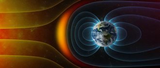
Migratory birds, such as cranes (Fig. 5), contain an organ capable of detecting changes in the Earth's magnetic field. Thanks to this, they orient themselves in space during flights to warmer climes.
Rice. 5. Migratory birds navigate by the Earth’s magnetic field
How can we detect the field without the help of animals?
To detect the electric field we will use an electric charge. Because the field acts with electric force on the charges placed in it.
And to detect the magnetic field, we can use a small magnet, or an iron object. Because the magnetic field will affect them.
Content
- 1. History
- 2 Classical fields 2.1 Newtonian gravity
- 2.2 Electromagnetism 2.2.1 Electrostatics
- 2.2.2 Magnetostatics
- 2.2.3 Electrodynamics
- 4.1 Field symmetries 4.1.1 Space-time symmetries
How are the fields indicated in the pictures?
Let's look at part of the world map. Let us pay attention to the fact that the areas of parts of the map are painted in different color shades (Fig. 6).
Rice. 6. Different elevation levels on the map are painted in different colors
Also, in one of the corners of the map you can see a multi-colored plate, similar to the one drawn on top of the map in the picture. A scale of heights and depths is drawn on it and, next to each shade, numbers are written indicating the height or depth in meters.
Note: Heights and depths on the ground are indicated using areas with different colors for clarity. The closer to red, the higher, and the closer to purple, the deeper.
Thin boundaries are drawn along the edges of the color areas; they limit areas that have the same height level. Such boundaries are called level lines.
Height or level is a scalar quantity. Therefore, we can say that with the help of colored areas and lines on their boundaries, a field is specified that describes the distribution of heights on the Earth's surface.
A scalar field can be represented using level lines.
Let us now recall the example with a magnet and a nail. At each point in the room you can draw a vector of the force with which the magnet attracts the iron nail (Fig. 7).
Rice. 7. Forces line up along certain lines, they are called field lines
The closer to the magnet, the greater the force of attraction, the longer the vectors. You can notice that the force vectors seem to be located along some lines. They are additionally shown as a dotted line in the figure. It can also be seen that these lines are curved.
Such lines along which the force vectors line up are called force lines. Force fields are vector.
Vector fields are represented using field lines. Force vectors are lined up along such lines. These lines have other names.
Relationship between scalar and vector fields
A scalar field can be associated with a vector field. Let's return to the example of marking heights on a map (Fig. 6). We know that there are areas on the map where there are sharp changes in elevation. In such areas there are several gradations of color shades, and areas with different colors are located more often in such places.
To indicate sharp changes in height, they came up with the use of a special vector - the gradient vector. It describes how quickly a scalar quantity changes, such as height on a map of an area.
This vector is denoted as follows:
\[\large \boxed{ \overrightarrow{grad \left( h \right)} }\]
Note: Gradient, from the word gradation - it can be translated as variety, or variability. For example, gradations of brightness have different shades of gray. In school physics, the gradient vector is usually not considered.
The gradient is directed towards the greatest increase in the physical quantity. And the length of the gradient vector is equal to the speed at which the physical value increases. magnitude in this direction.
There are different elevation differences in different parts of the map, somewhere the height changes faster, and somewhere more slowly. This means that in different areas of the terrain the gradient vector will have different lengths.
And if a vector quantity is distributed in space, then they say that such a physical field is given. quantities.
Thus, we obtained two related fields - a scalar height field and a vector gradient field, which describes the rate of change in height in different areas of the terrain.
For example, when describing the electric field, we will use two quantities - scalar - the potential of the electrostatic field and vector - the electric field strength. These quantities are related to each other using a gradient vector.
A Brief History of the Study of the Electric Field
It is believed that the engineer and physicist Charles Coulomb became the first researcher of the interaction of static charges. It was he who deduced the principle of their interaction. The foundation of Coulomb's research was Isaac Newton's theory of gravitational interaction.
Hans Oersted became the scientist who discovered the magnetic properties of electric current and field, and thanks to James Maxwell, we know that an electric field cannot exist without a magnetic field, which induces it. Maxwell also approved the concept of short-range electromagnetic interactions.
I advise you to read about the properties of the magnetic field.
Hans Oersted and James Maxwell
However, the electric field became the object of human research long before recent centuries. Thales of Miletus in the 7th century BC explored the nature of static electricity.
At the end of the 19th century, Joseph Thomson discovered the electron, a “living” example of the carrier of electricity. Years later, Ernst Rutherford proved the place in the structure of atoms where electrons are located.
Homogeneous and inhomogeneous fields
A field is homogeneous if at each point in space it has the same value of the distributed quantity.
For example, temperature at all points in space has the same value. Or, the electric field acts on a charge placed in it at all points in space with the same force.
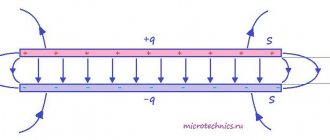
Homogeneous force fields are depicted by straight lines, the distance between which does not change (Fig. 8a).
Rice. 8. Lines of homogeneous – a) and inhomogeneous – b) fields
Distributed charges can create uniform fields. The electric field existing between two charged parallel planes is uniform.
If at different points in space the field acts on the test charge with different forces, then the field is called inhomogeneous. The lines of inhomogeneous fields are curved and the distance between them changes (Fig. 8b).
A field is inhomogeneous if at different points in space it has different values of the distributed magnitude.
For example, the field of a magnet is a non-uniform field because the force of the magnet increases as it approaches it. The electric field around a point charge is also non-uniform, because the force on the test charge increases with decreasing distance to the charge that created the field.
The strength of the field can be determined from the lines of force. The denser the field lines are in any area, the greater the magnitude of the field in that area.
Electric dipole
This term denotes an elementary collection of point charges that have systemic characteristics. A dipole is the sum of charges that are opposite, but equal in magnitude, and shifted from one another to a certain distance.
There are different dipoles, but physical science pays the most attention to point dipoles. This is the name given to dipoles, which are characterized by a negligible distance from a negative charge to a positive one. If, in theory, a collection of charges is divided into many parts, it can be considered as a system of electric dipoles.
Electric dipole moment
Examples of scalar fields
These are fields of distribution of scalar quantities - density, pressure, gravitational and electrostatic potentials, temperature, altitudes, etc.
Charge density field
When charges are distributed in three-dimensional space, we can talk about the density of such a distribution. Charge density is a scalar quantity. Its distribution defines a scalar field and is described by a scalar function.
Density field of bodies
If mass is distributed in space, then there is a mass distribution density. The body density is a scalar function; it defines a scalar field.
Sound wave pressure field
Let a sound wave be distributed in a gas or liquid. Sound waves are transverse waves. As the wave propagates in the gas or liquid, areas of condensation and rarefaction appear. Because the pressure fluctuates. It differs at different points in space. That is, it depends on the position of the point in space. When a scalar quantity, pressure, is distributed in space, its distribution is described by a scalar function. This function specifies a scalar field.
Gravitational potential field - distribution of potential energy
According to the law of universal gravitation, bodies with mass attract each other. And if there is interaction, then there is potential energy of such interaction. The distribution of potential energy is given by a scalar function; this function describes a scalar field and is called the gravitational potential.
Electric potential distribution field
Charges located at a certain distance attract or repel. This means that there is potential energy for their interaction. The energy distribution is described by the potential of a system of charged particles. Electric potential is a scalar function that describes a scalar field.
Examples of vector fields
These are fields of distribution of vector quantities - forces, velocities, etc.
Gravitational force field
The force of universal gravitation is a vector, which means the field describing the gravitational attraction of bodies will be vector.
Fluid flow velocity field
When a fluid flows, some parts of the fluid move faster than others. This means that the speeds of the liquid particles differ. The distribution of flow particle velocities can be described by a field. Velocity is a vector, which means that the field of fluid flow velocities is a vector field.
Field of Coulomb forces
We know that charges at rest attract or repel due to Coulomb forces. The forces of such interaction are distributed in space and set the field. This is an electrostatic field, it is a vector field of tension.
Magnetic force field
Moving charges interact due to magnetic fields. Magnetic field induction describes how the force of interaction changes in space. Therefore, the magnetic field induction is a vector function that specifies the vector magnetic field.
Note: Essentially, magnetic field induction is the force exerted on a moving charge by other moving charges.
Important Lessons
What can we learn from four examples showing class 0 waves?
(The equation of motion has one quantity, cw, and all waves in the corresponding field move at speed cw. Different Class 0 fields will have different values of cw). We can learn that the same field behavior can arise from physically different fields existing in physically different media. Despite their different origins, waves in the height field, in the lattice displacement field, in the magnetic orientation field and in the gas pressure field look identical in terms of fields. They satisfy the same type of equation of motion and the same numerical relationship between frequency and wavelength. The fine print: Strictly speaking, if you create waves of small enough wavelengths, you can still distinguish the behavior of different media. Once the wavelengths are equal to the distance between the atoms of a rope, or a crystal, or a magnet, the wave equations that the waves will satisfy will turn out to be more complex than what we have written down, and their details will allow us to distinguish the media from each other. But often in practical experiments we do not even come close to observing such effects.
The upshot of this is that the study of waves and their quanta associated with fields will not necessarily tell you what the medium is, or what the physical interpretation of the field is—what property of the medium it represents. And even if you somehow know that this field is a certain type - say, a pressure field - you usually still won't be able to tell, based on its behavior, the pressure of what exactly it represents. All you can learn by studying waves is whether the field belongs to class 0 or class 1, and what its cw value is; or find out that a field belongs to another class.
In some cases this is very bad; the field conveys only partial information about the environment. Sometimes this is quite convenient; a field is a more abstract and universal thing than the physical material it describes.
Therefore, the field does not define the environment, and its behavior is often independent of the details and properties of the environment. Which is why the question arises.
Can a physical field—with waves of quanta moving through space and carrying energy—exist without any medium to support it?
conclusions
- All quantities we measure can be divided into scalar ones, which have no direction, and vector ones, which have a direction.
- The field of a physical quantity is said to be given when this quantity is distributed in space.
- Not only scalar quantities, but also vector quantities can be distributed in space.
- If a scalar quantity is distributed in space, then the field is called scalar, and if it is a vector quantity, then the field is called vector.
- A field is stationary if it does not change over time. And if it changes, then the field is non-stationary.
- People may not sense all fields. But the field can be detected using bodies or instruments sensitive to these fields. For example, an electric field can be detected by its effect on charges.
- It is convenient to depict fields in the figures using special lines. It is convenient to denote scalar fields using level lines.
- Vector fields are depicted using lines along which vectors distributed in space are directed. Such lines are called lines of force, field strength lines, field induction lines.
- Vector and scalar fields can be linked. To do this, you can use a special vector - the gradient vector.
- A homogeneous field at every point in space has the same distributed value. Homogeneous force fields are depicted by straight lines, the distance between which is maintained.
- A non-uniform field at different points in space has different values of the distributed magnitude. Inhomogeneous fields are depicted by curved lines, the distance between them varies.
- The denser the field lines are in any area, the greater its value in that area.