Often in electronic circuits there is a need to generate different types of signals having different frequencies and shapes, such as square waves, square waves, triangular signals, sawtooth signals and various pulses.
These signals of various shapes can be used as synchronization signals, timing signals, or as trigger pulses. The first step is to understand the basic characteristics that describe electrical signals.
In technical terms, electrical signals are a visual representation of changes in voltage or current over time. That is, in fact, this is a graph of changes in voltage and current, where we plot time on the horizontal axis, and on the vertical axis we plot the voltage or current values at this point in time. There are many different types of electrical signals, but in general, they can all be divided into two main groups.
- Unipolar signals are electrical signals that are always positive or always negative and do not cross the horizontal axis. Unidirectional signals include square waves, clock pulses, and trigger pulses.
- Bipolar Signals - These electrical signals are also called alternating signals because they alternate between positive and negative values, constantly crossing zero. Bipolar signals have a periodic change in the sign of their amplitude. The most common bidirectional signal is the sine wave.
Whether unidirectional, bidirectional, symmetrical, asymmetrical, simple or complex, all electrical signals have three common characteristics:
- The period is the length of time after which the signal begins to repeat. This time value is also called the period time for sinusoids or the pulse width for square waves and is denoted by the letter T.
- Frequency is the number of times a signal repeats itself over a period of time equal to 1 second. Frequency is the reciprocal of the time period, ( *** QuickLaTeX cannot compile formula: f = 1/T *** Error message: Cannot connect to QuickLaTeX server: SSL certificate problem: certificate has expired Please make sure your server/PHP settings allow HTTP requests to external resources (“allow_url_fopen”, etc.) These links might help in finding a solution: https://wordpress.org/extend/plugins/core-control/ https://wordpress.org/support/topic/an -unexpected-http-error-occurred-during-the-api-request-on-wordpress-3?replies=37 ). The unit of frequency is Hertz (Hz). The frequency is 1 Hz and the signal repeats once every 1 second.
- Amplitude is the amount of change in the signal. It is measured in Volts (V) or Amperes (A), depending on which time dependence (voltage or current) we use.
Periodic signals
Periodic signals are the most common because they include sine waves. The alternating current in the outlet at home is a sinusoid, changing smoothly over time with a frequency of 50 Hz.
The time that passes between individual repetitions of a sinusoid cycle is called its period. In other words, this is the time it takes for the signal to start repeating.
The period can vary from fractions of a second to thousands of seconds, as it is related to its frequency. For example, a sine wave that takes 1 second to complete a cycle has a period of one second. Likewise, a sine wave that takes 5 seconds to complete a cycle has a period of 5 seconds, and so on.
So, the length of time it takes for a signal to complete a full cycle of its change before it repeats again is called the period of the signal and is measured in seconds. We can express the signal as the number of cycles T per second as shown in the figure below.
Links
- [standartgost.ru/%D0%93%D0%9E%D0%A1%D0%A2%2016465-70 GOST 16465-70].
| This is a preliminary article about electronics. You can help the project by adding to it. |
| : Incorrect or missing image | To improve this article it is desirable:
|
Sine wave
Period time is often measured in seconds (s), milliseconds (ms), and microseconds (µs).
For a sine waveform, the time period of the signal can also be expressed in degrees, or in radians, given that one complete cycle is equal to 360° (T = 360°), or, if in radians, then
*** QuickLaTeX cannot compile formula: 2 \pi *** Error message: Cannot connect to QuickLaTeX server: SSL certificate problem: certificate has expired Please make sure your server/PHP settings allow HTTP requests to external resources (“allow_url_fopen”, etc .) These links might help in finding a solution: https://wordpress.org/extend/plugins/core-control/ https://wordpress.org/support/topic/an-unexpected-http-error-occurred-during- the-api-request-on-wordpress-3?replies=37 (T = *** QuickLaTeX cannot compile formula: 2 \pi *** Error message: Cannot connect to QuickLaTeX server: SSL certificate problem: certificate has expired Please make make sure your server/PHP settings allow HTTP requests to external resources (“allow_url_fopen”, etc.) These links might help in finding a solution: https://wordpress.org/extend/plugins/core-control/ https://wordpress. org/support/topic/an-unexpected-http-error-occurred-during-the-api-request-on-wordpress-3?replies=37
).
Period and frequency are mathematically the reciprocals of each other. As the signal period time decreases, its frequency increases and vice versa.
The relationship between the signal period and its frequency:
*** QuickLaTeX cannot compile formula: f = \frac{1}{T} *** Error message: Cannot connect to QuickLaTeX server: SSL certificate problem: certificate has expired Please make sure your server/PHP settings allow HTTP requests to external resources (“allow_url_fopen”, etc.) These links might help in finding a solution: https://wordpress.org/extend/plugins/core-control/ https://wordpress.org/support/topic/an-unexpected-http -error-occurred-during-the-api-request-on-wordpress-3?replies=37
Hz
*** QuickLaTeX cannot compile formula: T = \frac{1}{f} *** Error message: Cannot connect to QuickLaTeX server: SSL certificate problem: certificate has expired Please make sure your server/PHP settings allow HTTP requests to external resources (“allow_url_fopen”, etc.) These links might help in finding a solution: https://wordpress.org/extend/plugins/core-control/ https://wordpress.org/support/topic/an-unexpected-http -error-occurred-during-the-api-request-on-wordpress-3?replies=37
c
One hertz is exactly equal to one cycle per second, but one hertz is a very small value, so you often see prefixes indicating the order of magnitude of the signal, such as kHz, MHz, GHz and even THz
| Prefix | Definition | Record | Period |
| Kilo | thousand | kHz | 1 ms |
| Mega | million | MHz | 1 µs |
| Giga | billion | GHz | 1 ns |
| Tera | trillion | THz | 1 ps |
Meander
Square waves are widely used in electronic circuits for timing and synchronization signals because they have a symmetrical square wave shape with equal half-cycle lengths. Almost all digital logic circuits use square wave signals at their inputs and outputs.
Since the shape of the meander is symmetrical, and each half of the cycle is the same, the duration of the positive part of the pulse is equal to the period of time when the pulse is negative (zero). For square waves used as timing signals in digital circuits, the duration of the positive pulse is called the period fill time.
For meander, filling time
*** QuickLaTeX cannot compile formula: \tau *** Error message: Cannot connect to QuickLaTeX server: SSL certificate problem: certificate has expired Please make sure your server/PHP settings allow HTTP requests to external resources (“allow_url_fopen”, etc. ) These links might help in finding a solution: https://wordpress.org/extend/plugins/core-control/ https://wordpress.org/support/topic/an-unexpected-http-error-occurred-during-the -api-request-on-wordpress-3?replies=37
equal to half the signal period. Since the frequency is equal to the reciprocal of the period, (1/T), then the frequency of the meander:
*** QuickLaTeX cannot compile formula: \ *** Error message: Cannot connect to QuickLaTeX server: SSL certificate problem: certificate has expired Please make sure your server/PHP settings allow HTTP requests to external resources (“allow_url_fopen”, etc.) These links might help in finding a solution: https://wordpress.org/extend/plugins/core-control/ https://wordpress.org/support/topic/an-unexpected-http-error-occurred-during-the- api-request-on-wordpress-3?replies=37
For example, for a signal with a fill time of 10 ms, its frequency is:
*** QuickLaTeX cannot compile formula: f = \frac{1}{(10+10) \cdot 10^{-3}c} = 50 *** Error message: Cannot connect to QuickLaTeX server: SSL certificate problem: certificate has expired Please make sure your server/PHP settings allow HTTP requests to external resources (“allow_url_fopen”, etc.) These links might help in finding a solution: https://wordpress.org/extend/plugins/core-control/ https: //wordpress.org/support/topic/an-unexpected-http-error-occurred-during-the-api-request-on-wordpress-3?replies=37
Hz
Square waves are used in digital systems to represent the logical “1” level by large values of its amplitude and the logical “0” level by small amplitude values.
If the filling time is not equal to 50% of the duration of its period, then such a signal already represents a more general case and is called a rectangular signal. If or if the time of the positive part of the signal period is short, then such a signal is an impulse.
Harmonic vibrations
There were several articles on the hub on the Fourier transform and about all sorts of beauties such as Digital Signal Processing (DSP), but it is completely unclear to the inexperienced user why all this is needed and where, and most importantly, how to apply it.
Frequency response of noise.
Personally, after reading these articles (for example, this one), it did not become clear to me what it was and why it was needed in real life, although it was interesting and beautiful. I want to not just look at beautiful pictures, but, so to speak, to feel in my gut what and how it works. And I will give a specific example with the generation and processing of sound files. It will be possible to listen to the sound, and look at its spectrum, and understand why this is so. The article will not be of interest to those who know the theory of functions of a complex variable, DSP and other scary topics. It is more for the curious, schoolchildren, students and those who sympathize with them :).
Let me make a reservation right away: I am not a mathematician, and I may even say many things incorrectly (correct them with a personal message), and I am writing this article based on my own experience and my own understanding of current processes. If you're ready, let's go.
A few words about materiel
If we remember our school mathematics course, we used a circle to plot the sine graph. In general, it turns out that rotational motion can be turned into a sine wave (like any harmonic oscillation). The best illustration of this process is given in Wikipedia
Harmonic vibrations
Those. in fact, the sine graph is obtained from the rotation of the vector, which is described by the formula:
f(x) = A sin (ωt + φ),
where A is the length of the vector (oscillation amplitude), φ is the initial angle (phase) of the vector at zero time, ω is the angular velocity of rotation, which is equal to:
ω=2 πf, where f is the frequency in Hertz.
As we see, knowing the signal frequency, amplitude and angle, we can construct a harmonic signal.
The magic begins when it turns out that the representation of absolutely any signal can be represented as a sum (often infinite) of different sinusoids. In other words, in the form of a Fourier series. I will give an example from the English Wikipedia. Let's take a sawtooth signal as an example.
Ramp signal
Its amount will be represented by the following formula:
If we add up one by one, take first n=1, then n=2, etc., we will see how our harmonic sinusoidal signal gradually turns into a saw:
This is probably most beautifully illustrated by one program I found on the Internet. It was already said above that the sine graph is a projection of a rotating vector, but what about more complex signals? This, oddly enough, is a projection of many rotating vectors, or rather their sum, and it all looks like this:
Vector drawing saw.
In general, I recommend going to the link yourself and trying to play with the parameters yourself and see how the signal changes. IMHO I have never seen a more visual toy for understanding.
It should also be noted that there is an inverse procedure that allows you to obtain frequency, amplitude and initial phase (angle) from a given signal, which is called the Fourier Transform.
Fourier series expansion of some well-known periodic functions (from here)
I won’t dwell on it in detail, but I will show how it can be applied in life. In the bibliography I will recommend where you can read more about the materiel.
Let's move on to practical exercises!
It seems to me that every student asks a question while sitting at a lecture, for example on mathematics: why do I need all this nonsense? And as a rule, having not found an answer in the foreseeable future, unfortunately, he loses interest in the subject. Therefore, I will immediately show the practical application of this knowledge, and you will already master this knowledge yourself :).
I will implement everything further on my own. I did everything, of course, under Linux, but did not use any specifics; in theory, the program will compile and run under other platforms.
First, let's write a program to generate an audio file. The wav file was taken as the simplest one. You can read about its structure here. In short, the structure of a wav file is described as follows: a header that describes the file format, and then there is (in our case) an array of 16-bit data (pointer) with a length of: sampling_frequency*t seconds or 44100*t pieces.
An example was taken here to generate a sound file. I modified it a little, corrected errors, and the final version with my edits is now on Github here
github.com/dlinyj/generate_wav
Let's generate a two-second sound file with a pure sine wave with a frequency of 100 Hz. To do this, we modify the program as follows:
#define S_RATE (44100) //sampling frequency #define BUF_SIZE (S_RATE*10) /* 2 second buffer */ …. int main(int argc, char * argv[]) { ... float amplitude = 32000; //take the maximum possible amplitude float freq_Hz = 100; //signal frequency /* fill buffer with a sine wave */ for (i=0; i
Please note that the formula for pure sine corresponds to the one we discussed above. The amplitude of 32000 (32767 could have been taken) corresponds to the value that a 16-bit number can take (from minus 32767 to plus 32767).
As a result, we get the following file (you can even listen to it with any sound reproducing program). Let's open this audacity file and see that the signal graph actually corresponds to a pure sine wave:
Pure tube sine
Let's look at the spectrum of this sine (Analysis->Plot spectrum)
Spectrum graph
A clear peak is visible at 100 Hz (logarithmic scale). What is spectrum? This is the amplitude-frequency characteristic. There is also a phase-frequency characteristic. If you remember, I said above that to build a signal you need to know its frequency, amplitude and phase? So, you can get these parameters from the signal. In this case, we have a graph of frequencies corresponding to amplitude, and the amplitude is not in real units, but in Decibels.
A value expressed in decibels is numerically equal to the decimal logarithm of the dimensionless ratio of a physical quantity to the physical quantity of the same name, taken as the original, multiplied by ten.
In this case, simply the logarithm of the amplitude multiplied by 10. The logarithmic scale is convenient to use when working with signals.
To be honest, I don’t really like the spectrum analyzer in this program, so I decided to write my own with blackjack and whores, especially since it’s not difficult.
We are writing our own spectrum analyzer
This might get boring, so you can skip straight to the next chapter.
Since I understand perfectly well that there is no point in posting foot wraps of code here, those who are really interested will find it and dig into it themselves, and those who are not interested will be bored, I will only focus on the main points of writing a spectrum analyzer for a wav file.
First, we need to read the wav file. There you need to read the header to understand what the file contains. I did not implement a sea of options for reading this file, but settled on only one. The file reading example was taken from here with virtually no changes, IMHO it’s an excellent example. There is also an implementation in Python.
The next thing we need is a fast Fourier transform. This is the same transformation that allows you to obtain a vector a
original signals. Don’t let this scare you for now, I’ll explain later. Again, I didn’t reinvent the wheel, but took a ready-made example from here.
I understand that in order to explain how the program works, it is necessary to explain what the fast Fourier transform is, and this is at least one more article.
First, let's allocate the arrays:
c = calloc(size_array*2, sizeof(float)); // array of rotation factors in = calloc(size_array*2, sizeof(float)); //input array out = calloc(size_array*2, sizeof(float)); //output array
Let me just say that in the program we read data into an array of length size_array (which we take from the header of the wav file).
while( fread(&value,sizeof(value),1,wav) ) { in[j]=(float)value; j+=2; if (j > 2*size_array) break; }
The array for fast Fourier transform must be a sequence {re[0], im[0], re[1], im[1],… re[fft_size-1], im[fft_size-1]}, where fft_size=1 << p — number of FFT points. I’ll explain it in normal language: this is an array of complex numbers. I’m even afraid to imagine where the complex Fourier transform is used, but in our case, our imaginary part is equal to zero, and the real part is equal to the value of each point of the array. Another feature of the fast Fourier transform is that it calculates arrays that are multiples only of powers of two. As a result, we must calculate the minimum power of two:
int p2=(int)(log2(header.bytes_in_data/header.bytes_by_capture));
The logarithm of the number of bytes in the data divided by the number of bytes at one point.
After this, we calculate the rotation factors:
fft_make(p2,c); // function for calculating rotation factors for FFT (the first parameter is a power of two, the second is an allocated array of rotation factors).
And we feed our just array into the Fourier transformer:
fft_calc(p2, c, in, out, 1); //(one means we are getting a normalized array).
At the output we get complex numbers of the form {re[0], im[0], re[1], im[1],... re[fft_size-1], im[fft_size-1]}. For those who don’t know what a complex number is, I’ll explain. It’s not for nothing that I started this article with a bunch of rotating vectors and a bunch of GIFs. So, a vector on the complex plane is determined by the real coordinate a1 and the imaginary coordinate a2. Or length (this is amplitude Am for us) and angle Psi (phase).
Vector on the complex plane
Please note that size_array=2^p2. The first point of the array corresponds to a frequency of 0 Hz (constant), the last point corresponds to the sampling frequency, namely 44100 Hz. As a result, we must calculate the frequency corresponding to each point, which will differ by the delta frequency:
double delta=((float)header.frequency)/(float)size_array; //sampling frequency per array size.
Allocation of the amplitude array:
double * ampl; ampl = calloc(size_array*2, sizeof(double));
And look at the picture: amplitude is the length of the vector. And we have its projections onto the real and imaginary axis. As a result, we will have a right triangle, and here we remember the Pythagorean theorem, and count the length of each vector, and immediately write it into a text file:
for(i=0;i<(size_array);i+=2) { fprintf(logfile,"%.6f %f\n",cur_freq, (sqrt(out
*out +out[i+1]*out[i +1])));
cur_freq+=delta; } As a result, we get a file that looks something like this: ... 11.439514 10.943008 11.607742 56.649738 11.775970 15.652428 11.944199 21.872342 12.112427 30.635371 12.280655 30 .329171 12.448883 11.932371 12.617111 20.777617 ... The final version of the program lives on GitHub here: github.com/dlinyj/fft
Let's try!
Now we feed the resulting program that sine sound file
./fft_an ../generate_wav/sin\ 100\ Hz.wav format: 16 bits, PCM uncompressed, channel 1, freq 44100, 88200 bytes per sec, 2 bytes by capture, 2 bits per sample, 882000 bytes in data chunk= 441000 log2=18 size array=262144 wav format Max Freq = 99.928 , amp =7216.136
And we get a text file of the frequency response. We build its graph using a gnuplot
Script for construction:
#! /usr/bin/gnuplot -persist set terminal postscript eps enhanced color solid set output "result.ps" #set terminal png size 800, 600 #set output "result.png" set grid xtics ytics set log xy set xlabel "Freq, Hz" set ylabel "Amp, dB" set xrange [1:22050] #set yrange [0.00001:100000] plot "test.txt" using 1:2 title "AFC" with lines linestyle 1
Please note the limitation in the script on the number of points in X: set xrange [1:22050]. Our sampling frequency is 44100, and if we recall Kotelnikov’s theorem, then the signal frequency cannot be higher than half the sampling frequency, therefore we are not interested in a signal above 22050 Hz. Why this is so, I advise you to read in specialized literature. So (drumroll), run the script and see:
Spectrum of our signal
Note the sharp peak at 100 Hz. Don't forget that the axes are on a logarithmic scale! The wool on the right is what I think are Fourier transform errors (windows come to mind here).
Let's indulge?
Come on! Let's look at the spectra of other signals!
There is noise around...
First, let's plot the noise spectrum.
The topic is about noise, random signals, etc. worthy of a separate course. But we will touch on it lightly. Let's modify our wav file generation program and add one procedure: double d_random(double min, double max) { return min + (max - min) / RAND_MAX * rand(); } it will generate a random number in the given range. As a result, main will look like this:
int main(int argc, char * argv[]) { int i; float amplitude = 32000; srand((unsigned int)time(0)); //initialize the random number generator for (i=0; i
Let's generate a file (I recommend listening to it). Let's look at it in audacity.
Signal in audacity
Let's look at the spectrum in the audacity program.
Range
And let's look at the spectrum using our program:
Our spectrum
I would like to draw your attention to a very interesting fact and feature of noise - it contains the spectra of all harmonics. As can be seen from the graph, the spectrum is quite even. Typically, white noise is used for frequency analysis of bandwidth, such as audio equipment. There are other types of noise: pink, blue and others
. Homework is to find out how they differ.
What about compote?
Now let's look at another interesting signal - a meander. I gave above a table of expansions of various signals in Fourier series, you look at how the meander is expanded, write it down on a piece of paper, and we will continue.
To generate a square wave with a frequency of 25 Hz, we once again modify our wav file generator:
int main(int argc, char * argv[]) { int i; short int meandr_value=32767; /* fill buffer with a sine wave */ for (i=0; i
As a result, we get an audio file (again, I advise you to listen), which you should immediately watch in audacity
His Majesty is the meander or meander of a healthy person
Let's not languish and look at its spectrum:
Meander spectrum
It’s not very clear yet what it is... Let’s take a look at the first few harmonics:
First harmonics
It's a completely different matter! Well, let's look at the sign. Look, we only have 1, 3, 5, etc., i.e. odd harmonics. We see that our first harmonic is 25 Hz, the next (third) is 75 Hz, then 125 Hz, etc., while our amplitude gradually decreases. Theory meets practice! Now attention! In real life, a square wave signal has an infinite sum of harmonics of higher and higher frequencies, but as a rule, real electrical circuits cannot pass frequencies above a certain frequency (due to the inductance and capacitance of the tracks). As a result, you can often see the following signal on the oscilloscope screen:
Smoker's meander
This picture is just like the picture from Wikipedia, where for the example of a meander, not all frequencies are taken, but only the first few.
The sum of the first harmonics, and how the signal changes
The meander is also actively used in radio engineering (it must be said that this is the basis of all digital technology), and it is worth understanding that with long circuits it can be filtered so that the mother does not recognize it. It is also used to check the frequency response of various devices. Another interesting fact is that TV jammers worked precisely on the principle of higher harmonics, when the microcircuit itself generated a meander of tens of MHz, and its higher harmonics could have frequencies of hundreds of MHz, exactly at the operating frequency of the TV, and the higher harmonics successfully jammed the TV broadcast signal.
In general, the topic of such experiments is endless, and you can now continue it yourself.
Reading Suggestions
Book
For those who don’t understand what we’re doing here, or vice versa, for those who understand but want to understand it even better, as well as for students studying DSP, I highly recommend this book. This is a DSP for dummies, which is the author of this post. There, complex concepts are explained in a language accessible even to a child.
Conclusion
In conclusion, I would like to say that mathematics is the queen of sciences, but without real application, many people lose interest in it. I hope this post will encourage you to study such a wonderful subject as signal processing, and analog circuitry in general (plug your ears so your brains don’t leak out!). Good luck!
Square wave
Rectangular signals differ from meanders in that the durations of the positive and negative parts of the period are not equal. Square wave signals are therefore classified as single-ended signals.
In this case, I have depicted a signal that takes only positive values, although, in general, negative signal values can be significantly below the zero mark.
In the example shown, the duration of the positive pulse is longer than the duration of the negative one, although this is not necessary. The main thing is that the signal shape is rectangular.
Signal repetition period ratio
*** QuickLaTeX cannot compile formula: T *** Error message: Cannot connect to QuickLaTeX server: SSL certificate problem: certificate has expired Please make sure your server/PHP settings allow HTTP requests to external resources (“allow_url_fopen”, etc.) These links might help in finding a solution: https://wordpress.org/extend/plugins/core-control/ https://wordpress.org/support/topic/an-unexpected-http-error-occurred-during-the- api-request-on-wordpress-3?replies=37 , to the duration of the positive pulse *** QuickLaTeX cannot compile formula: \tau *** Error message: Cannot connect to QuickLaTeX server: SSL certificate problem: certificate has expired Please make sure your server/PHP settings allow HTTP requests to external resources (“allow_url_fopen”, etc.) These links might help in finding a solution: https://wordpress.org/extend/plugins/core-control/ https://wordpress.org /support/topic/an-unexpected-http-error-occurred-during-the-api-request-on-wordpress-3?replies=37
, is called duty cycle:
*** QuickLaTeX cannot compile formula: \ *** Error message: Cannot connect to QuickLaTeX server: SSL certificate problem: certificate has expired Please make sure your server/PHP settings allow HTTP requests to external resources (“allow_url_fopen”, etc.) These links might help in finding a solution: https://wordpress.org/extend/plugins/core-control/ https://wordpress.org/support/topic/an-unexpected-http-error-occurred-during-the- api-request-on-wordpress-3?replies=37
The reverse duty cycle value is called the duty cycle:
*** QuickLaTeX cannot compile formula: \ *** Error message: Cannot connect to QuickLaTeX server: SSL certificate problem: certificate has expired Please make sure your server/PHP settings allow HTTP requests to external resources (“allow_url_fopen”, etc.) These links might help in finding a solution: https://wordpress.org/extend/plugins/core-control/ https://wordpress.org/support/topic/an-unexpected-http-error-occurred-during-the- api-request-on-wordpress-3?replies=37
Calculation example
Let there be a rectangular signal with a pulse duration of 10 ms and a duty cycle of 25%. It is necessary to find the frequency of this signal.
The duty cycle is 25% or ¼, and coincides with the pulse width, which is 10ms. Thus, the signal period should be equal to: 10ms (25%) + 30ms (75%) = 40ms (100%).
*** QuickLaTeX cannot compile formula: f = \frac{1}{T} = \frac{1}{(10 + 30) \cdot 10^{-3}c} = 25 *** Error message: Cannot connect to QuickLaTeX server: SSL certificate problem: certificate has expired Please make sure your server/PHP settings allow HTTP requests to external resources (“allow_url_fopen”, etc.) These links might help in finding a solution: https://wordpress.org/extend /plugins/core-control/ https://wordpress.org/support/topic/an-unexpected-http-error-occurred-during-the-api-request-on-wordpress-3?replies=37
Hz
Square wave signals can be used to control the amount of power delivered to a load, such as a lamp or motor, by varying the duty cycle of the signal. The higher the duty cycle, the greater the average amount of energy must be supplied to the load, and, accordingly, a lower duty cycle means a lower average amount of energy supplied to the load. A great example of this is the use of pulse width modulation in speed controllers. The term pulse width modulation (PWM) literally means “change in pulse width.”
PWM signal
Hardware
To generate a PWM signal with a given filling, there is a standard function analogWrite(pin, duty), discussed in more detail in the lesson about the PWM signal, and the frequency can be changed by reconfiguring the timer, as in the lesson about increasing the PWM frequency. In fact, timers allow you to configure the PWM signal with a more precise or higher frequency and different fill ranges (up to 10 bits), but this is not provided in the Arduino core. If you need this, you can use the GyverPWM library. Example:
pinMode(10, OUTPUT); // run PWM on D10 with a frequency of 150'000 Hz, FAST_PWM mode PWM_frequency(10, 150000, FAST_PWM);
Software PWM
Software generation of a PWM signal can be useful if there is not enough extra timer or the PWM frequency is low and will not affect the rest of the code, but it will not affect it. The PWM signal on the “millis” can be organized in this way, switching the output over two periods:
Soft PWM on millis()
The PWMgen(fill) function in this implementation should be called as often as possible in the main program loop:
#define PWM_PRD 20 // PWM period, ms #define PWM_PIN 13 // PWM pin void setup() { pinMode(PWM_PIN, OUTPUT); } void loop() { PWMgen(analogRead(0) / 4); // take the PWM value from A0, 0.. 255 } void PWMgen(byte duty) { static uint32_t tmr; static bool flag; if (duty == 0) digitalWrite(PWM_PIN, LOW); else if (duty == 255) digitalWrite(PWM_PIN, HIGH); else { int prd = (PWM_PRD * duty) >> 8; // equivalent / 255 if (millis() - tmr >= (flag ? prd : PWM_PRD - prd)) { tmr = millis(); digitalWrite(PWM_PIN, flag = !flag); } } }
Here, on each call, we calculate a new switching period, spending some time on this. You can count the period in a separate function, and generate the PWM itself separately. The implementation can be viewed in the PWMrelay library.
Semi-hardware PWM
You can reduce the load on the processor by assigning time to a hardware timer. Examples based on GyverTimers (for ATmega328, 2560):
8 bit PWM
// PWM frequency = ~ (call frequency tick / 256); #define PWM_FREQ 100 // PWM frequency #define PWM_PIN 13 // PWM pin #include // connect the volatile hardware timer library uint8_t pwm_duty = 0; // variable for storing PWM filling 0-255 volatile uint8_t counter = 0; // analogue of the timer counting register void setup() { Timer2.setFrequency(256L * PWM_FREQ); // interrupt frequency Timer2.enableISR(); // enable timer interrupts pinMode(PWM_PIN, OUTPUT); // pin as output } void loop() { // set the duty cycle of the PWM potentiometer from pin A0 pwm_duty = analogRead(0) / 4; // 1023 -> 255 // delay setting the value to avoid jumps delay(100); } // timer interrupt ISR(TIMER2_A) { if (!pwm_duty) digitalWrite(PWM_PIN, LOW); // PWM filling == 0 else { if (!counter) digitalWrite(PWM_PIN, HIGH); // when the counter is reset HIGH else if (counter == pwm_duty) digitalWrite(PWM_PIN, LOW); // if there is a match LOW counter++; } }
Setting the bit depth
// PWM frequency = ~ (tick call frequency / (PWM depth + 1)); #define PWM_DEPTH 100 // PWM bit depth #define PWM_PIN 13 // PWM pin #include // connect the volatile hardware timer library uint8_t pwm_duty = 0; // variable for storing PWM filling 0-255 volatile uint8_t counter = 0; // analogue of the timer counting register void setup() { Timer2.setPeriod(10); // timer interrupts with a frequency of 100 kHz Timer2.enableISR(); // enable timer 2 interrupts pinMode(PWM_PIN, OUTPUT); // set the pin to the output } void loop() { // get the PWM filling from potentiometer A0 pwm_duty = map(analogRead(A0), 0, 1023, 0, PWM_DEPTH); // delay setting the value to avoid jumps delay(100); } ISR(TIMER2_A) { if (!pwm_duty) digitalWrite(PWM_PIN, LOW); // PWM filling == 0 else { if (!counter) digitalWrite(PWM_PIN, HIGH); // when the counter is reset HIGH else if (counter == pwm_duty) digitalWrite(PWM_PIN, LOW); // if there is a match LOW if (++counter > PWM_DEPTH) counter = 0; // check for overflow } }
As you know, digitalWrite() is a very heavy and long function, and to generate soft PWM it is recommended to replace it with something faster, for example, direct access to a register or this construction (for ATmega328p):
void digitalWriteFast(uint8_t pin, bool x) { if (pin < { bitWrite(PORTD, pin, x); } else if (pin < 14) { bitWrite(PORTB, (pin - 8), x); } else if ( pin < 20) { bitWrite(PORTC, (pin - 14), x); } }
If the number of standard PWM outputs is not enough, you can raise the semi-hardware PWM on the timer by several pins at once:
Multichannel software PWM
#define PWM_FREQ 100 // PWM frequency const uint8_t pwm_pins[] = {2, 3, 4, 5}; // pins #include // connect the hardware timer library const uint8_t PWM_PINS = sizeof(pwm_pins); volatile uint8_t pwm_duty[PWM_PINS]; // variable for storing PWM filling 0-255 volatile uint8_t counter; // counter void setup() { Timer2.setFrequency(256L * PWM_FREQ); // timer interrupts Timer2.enableISR(); // enable timer 2 interrupts // set pins to the output for (int i = 0; i < PWM_PINS; i++) pinMode(pwm_pins , OUTPUT); // filling pwm_duty[0] = 10; pwm_duty[1] = 20; pwm_duty[2] = 128; pwm_duty[3] = 128; } void loop() { } // timer interrupt ISR(TIMER2_A) { for (int i = 0; i < PWM_PINS; i++) { if (!pwm_duty ) digitalWrite(pwm_pins , LOW); // PWM filling == 0 else { if (!counter) digitalWrite(pwm_pins , HIGH); // when the counter is reset HIGH else if (counter == pwm_duty ) digitalWrite(pwm_pins , LOW); // if there is a match LOW } } counter++; }
This algorithm is not the most optimal; a more interesting one can be found in GyverHacks.
Note : all three algorithms use a match check with counter == pwm_duty. This greatly reduces the use of CPU time in the interrupt, but with a sharp decrease in filling, it can lead to single “flashes” of filling to the maximum, since the condition is not met. For smoother operation, you can make counter >= pwm_duty, then the condition will be “adjusted” to the new filling value each time, but the pin will be set on every tick!
You can introduce PWM fill buffering and take a new value only when the counter is zero, this will solve the problem:
Buffered PWM
// soft PWM with buffering #define PWM_FREQ 100 // PWM frequency #define PWM_PIN 13 // PWM pin #include // connect the volatile hardware timer library uint8_t pwm_duty = 0; // variable for storing PWM filling 0-255 volatile uint8_t counter = 0; // analogue of the volatile timer counting register uint8_t real_duty = 0; void setup() { Timer2.setFrequency(256L * PWM_FREQ); // interrupt frequency Timer2.enableISR(); // enable timer interrupts pinMode(PWM_PIN, OUTPUT); // pin as output } void loop() { // set the duty cycle of the PWM potentiometer from pin A0 pwm_duty = analogRead(0) / 4; // 1023 -> 255 } // timer interrupt ISR(TIMER2_A) { if (!pwm_duty) digitalWrite(PWM_PIN, LOW); // filling PWM == 0 else { if (!counter) { // at counter == 0 digitalWrite(PWM_PIN, HIGH); // HIGH real_duty = pwm_duty; // take from the “buffer” } else if (counter == real_duty) digitalWrite(PWM_PIN, LOW); // if there is a match LOW counter++; } }
You can apply buffering to other algorithms.
Servo Library
As you know, RC servos are controlled using a PWM signal with a frequency of ~50 Hz and a pulse duration of ~500 to ~2500 microseconds. The standard Servo.h library implements the generation of a semi-hardware PWM signal, and the number of pins can be changed during operation. The library can be used as PWM generation if its parameters are suitable for use.
Triangle signals
Triangle signals are generally bidirectional, non-sinusoidal signals that oscillate between positive and negative peak values. A triangle waveform is a relatively slowly rising and falling voltage at a constant frequency. The rate at which the voltage changes direction is equal for both halves of the period, as shown below.
Typically, for triangular signals, the duration of the signal's rise is equal to the duration of its fall, thereby giving a 50% duty cycle. By setting the amplitude and frequency of the signal, we can determine the average value of its amplitude.
In the case of an asymmetrical triangular waveform, which we can obtain by changing the rate of rise and fall by different amounts, we have another type of signal known as a sawtooth waveform.
Conversation seven. Square wave signals. Limitation. Differentiation and integration
Neznaykin is extremely worried: he is accustomed to low-frequency techniques, where it is necessary to preserve the shape of the signal, and now, watching how Lyuboznaykin systematically deforms the signal, he is completely confused. Neznaykin begins to learn what limiting a signal from above is, how to turn a slow voltage change into an abrupt one, then he comprehends the secrets of differentiating and integrating circuits. The inevitable happens (against his wishes and his well-known horror of mathematics) - he is forced to swallow the (simplified!) definition of derivatives and integrals... and he realizes that the equation is much simpler than usually thought.
Square wave signals. Limitation. Differentiation and integration
Neznaykin - Dear Lyuboznaykin, last time I forgot to ask you one question.
Please tell me how accurately the various “super amplifiers” you told me about reproduce signals?
Lyuboznaykin - The reproduction accuracy is excellent in all systems assembled using a cathode or emitter follower circuit and, especially, in a “super emitter follower” on two mutually complementary transistors, since this circuit is characterized by deep negative feedback.
It goes without saying that you can achieve this fidelity only if you do not overload the circuit, that is, do not force it to output the highest current or the highest voltage, but in industrial electronics in many cases linearity is not the main requirement, presented to the amplifier, sometimes even vice versa...
Intentional misstatements
N. - That's how it is! So this means that the signal is deformed, relying on chance or due to perversity?
L. - Yes, the signal is deformed, but not by chance. As for perversion, you can and probably will suggest that I found the AZSOPD (Association of Signal Defenders from Vicious Deformation).
N. - I hope that you will join this association. But how can warped signals create undistorted sound?
L. - This time, get rid of your ideas about soundification and musicality from your head. Sound reproduction is one of the areas of application of radio electronics, but it by no means exhausts all radio electronics, just as electricity serves not only to power electric stoves. The voltage from your amplifier's output can drive more than just your loudspeaker. And, if you want it, for example, to turn on a relay, does the voltage have to be sinusoidal?
N. - I agree. What deformations will you subject the signal to?
L. - We will start by limiting the signal from above, since this practical method allows us to equalize the magnitude of signals with different amplitudes. This problem can be successfully solved by using a simple diode. As you can see, shown in Fig. 53 circuit will only pass the positive part of the UBX input signal to the output.
N. - This is easy to understand. But why was resistor R needed here?
L. - His role is not so obvious. Imagine that some load using voltage is connected to the output
limiter Fig. 53. Limiter. Only the positive part of the voltage supplied to the input passes to the output.
limiter Fig. 54. Limiter with a diode connected in parallel, short-circuiting the circuit for the negative part of the input voltage UBblx.
Ramp signal
A ramp wave is another type of periodic waveform. As the name suggests, the shape of this signal resembles the teeth of a saw. A sawtooth signal can be a mirror image of itself, having either a slow rise but a very steep fall, or an extremely steep, nearly vertical rise and a slow fall.
The slow-rising ramp wave is the more common of the two waveform types, being almost perfectly linear. The sawtooth waveform is generated by most function generators and consists of a fundamental frequency (f) and even harmonics. This means, from a practical point of view, that it is rich in harmonics, and in the case of, for example, music synthesizers, produces high-quality sound without distortion for musicians.