Everyone knows that the effective voltage in the socket is 220 Volts (230 according to the new standards, but for this topic this does not really matter). This can be easily checked using a multimeter, which will measure the potential difference between the phase and the working neutral conductor. That is, under ideal conditions, the potential on the neutral wire is 0, and on the phase wire 220 Volts. In fact, everything is a little different - alternating current has a sinusoidal shape with a potential at peaks of 310 and -310 Volts (amplitude voltage). In order to see this, you need to use an oscilloscope.
Definition
Root mean square (RMS) is a static measure of a variable. This is useful if the function alternates between positive and negative exponents (sine waves). Here we have the square root of the arithmetic mean of squares. In the case of a set of values n (x1, x2, …., xn), the RMS is determined by the formula:
The corresponding formula for a continuous function f (t) calculated on the interval T1 ≤ t ≤ T2:
RMS current for the function over the entire time:
The rms voltage value during the periodic function is equal to the RMS value of one period.
What is the average value of AC voltage?
Another parameter of alternating voltage that characterizes it is the average value of alternating voltage. Unlike the effective value of alternating voltage, which characterizes the operation of alternating voltage, the average value of voltage characterizes the amount of electricity that moves from one point in the circuit to another under the influence of alternating voltage. The average voltage value over a period is determined by the following expression
where T is the period of alternating voltage,
fu(t) – functional dependence of voltage on time.
Thus, the average value of the alternating voltage will be numerically equal to the height of a rectangle with a base T, the area of which is equal to the area limited by the function fu(t) and the Ox axis for the period T.
Average value of alternating voltage.
In the case of a sinusoidal function, we can only talk about the average value over a half-cycle, since during the entire period the positive half-wave is compensated by the negative half-wave, and then the average voltage over the period will be zero.
Thus, the average value of the sinusoidal alternating voltage over the half-cycle T/2 will be equal to
where Um is the maximum voltage value or amplitude,
ω – angular frequency, rate of change of argument (angle).
Application to voltage and current
Let's take a look at a sinusoidally varying voltage:
(a) – Constant voltage and current remain stable. (b) – Graph of voltage and current versus time for 60 Hz AC power. The voltage and current are sinusoidal and in phase for a simple resistance circuit. Frequencies and peak voltages vary greatly
V = V0sin (2πft), where V is the voltage at an instant, V0 is the peak voltage, f is the frequency in Hz. For this simple resistance circuit, I = V/R, so the AC current looks like:
I = I0sin (2πft), where I is the current at an instant and I0 = V0/R is the peak current. Now, using the above definition, we derive the rms voltage and current. First of all we have
Here we have replaced 2πf with ω. Since V0 is a constant, we can expand it by its square root and use the trigonometric formula to replace the square of the sine function.
Integrating what was written:
Since the interval represents an integer number of complete cycles, the terms are canceled, leaving:
You will also understand that RMS can be expressed through
What is AC rms voltage?
As I wrote above, one of the main parameters of alternating voltage is the amplitude Um, however, it is not convenient to use this value in calculations, since the time interval during which the voltage value u is equal to the amplitude Um is negligible compared to the period T of the voltage. Using the instantaneous voltage value u is also not very convenient due to the large volume of calculations. Then the question arises, what value of alternating voltage should be used in the calculations?
To solve this issue, it is necessary to turn to the energy that is released under the influence of alternating voltage and compare it with the energy that is released under the influence of constant voltage. To solve this issue, let us turn to the Joule–Lenz law for constant voltage
For alternating voltage, the instantaneous value of the released energy will be
where u is the instantaneous voltage value
Then the amount of energy for the full period from t0 = 0 to t1 = T will be
By equating the expressions for the amount of energy at alternating voltage and constant voltage and expressing the resulting expression in terms of constant voltage, we obtain the effective value of alternating voltage
The resulting expression allows you to calculate the effective value of voltage U for a periodic alternating voltage of any shape. From the above, we can conclude that the effective value of an alternating voltage is called a constant voltage that, in the same time and at the same resistance, releases the same energy that is released by a given alternating voltage.
Effective value of sinusoidal voltage.
Let's calculate the effective value of the sinusoidal voltage
It is worth noting that all voltages of electrical devices are determined, as a rule, by the effective voltage value.
To determine the amplitude value of the sinusoidal voltage, it is necessary to transform the resulting expression
Thus, if we have U = 230 V in the socket, therefore, the amplitude value of this voltage
Effective voltage is also called effective voltage and root mean square voltage.
We've sorted out the effective voltage, now let's look at the average voltage.
Light bulb and constant voltage
For experiments we will also need a simple 12 Volt car incandescent lamp
Here are its characteristics: operating voltage U = 12 Volts, power P = 21 Watts.
Therefore, knowing the power and voltage of the lamp, you can find out how much current the light bulb will consume. From the formula P=IU, where I is the current strength, you can find I. This means I=P/U=21/12=1.75 Amperes.
Okay, we've sorted out the light bulb. Let's light it up. To do this, set the operating voltage for our lamp on our power supply
We supply voltage from the power supply to the lamp and voila!
We measure the voltage at the alligator terminals of the power supply using a multimeter. Exactly 12 Volts, as expected.
We connect our oscilloscope to the same terminals
Let's look at the oscillogram:
Do you see a straight line? This is a DC voltage oscillogram. Over time, our tension remains the same as it was and does not change. If you do the math, you can figure out what the voltage is. Since one cell has 5 Volts (pictured below left), this means our voltage is 12 Volts. I also plotted this value on the oscilloscope display in the very bottom left corner: 12.03 Volts. That's right.
We measure the current strength. You can learn how to correctly measure the current in a circuit by reading the article How to measure current and voltage with a multimeter?
We got 1.72 Amperes. And as you remember, our calculated value was 1.75 Amps. I think the blame can be shifted to the error of the device or to the light bulb 
Sinusoid of effective and amplitude voltage
It is clear that this material is more aimed at a simple audience, who not only do not have an oscilloscope, but probably not everyone even has a multimeter. Therefore, all examples will be taken from the Electronics Workbench environment, which is accessible to everyone.
And the first thing we need to look at is the phase voltage sine wave from the outlet. To do this, we will draw a three-phase network in the program and connect the oscilloscope to one of the phases:
As can be seen with a voltmeter reading of 219.4 Volts between one of the phases and the PEN conductor, the oscilloscope showed a sine wave with an amplitude of 309.1 Volts. This voltage value is called maximum (amplitude). And 219.4 Volts, which the voltmeter shows, is the effective voltage. It is also called root mean square or effective. And before we move on to consider this feature, let’s briefly, in simple words, go through the drawn diagram of a three-phase network and understand the nature of the sinusoid.
Let's start with the diagram:
- From left to right - three AC voltage sources with phase angles of 0, 120, 240 degrees and connected by a star.
- The 4 Ohm resistor is the grounding of the transformer neutral.
- Resistors of 0.8 ohms are the conditional resistance of the wires, depending on the cross-section of the wire and the length of the line.
- Resistors 15, 10 and 20 Ohms - load of consumers in three phases.
- An oscilloscope is connected to one of the phases, showing an amplitude of 309.1 Volts.
Now let's look at a sinusoid. Alternating voltage, in contrast to constant voltage, the graph of which is straight on an oscilloscope, continuously changes both in magnitude and direction. Moreover, these changes occur periodically, that is, they are exactly repeated at regular intervals.
Alternating voltage is generated at power plants and reaches the end consumer through step-up and step-down distribution transformers. In this case, the transformation along the path does not affect the voltage sinusoid in any way.
Calculation of effective value
As an example, let's calculate the root mean square value of the sinusoidal voltage.
Let us write the expression U rms
using the integral of the function
U = U ampsin(t)
for one period 2
π
:
Let's take out U amp
from under the radical sign. Let's use the table integral, rewrite and solve the last expression using the Newton-Leibniz formula:
Since sin(2 π
), sin(4
π
) and sin(0) are equal to zero, we calculate the RMS of the sinusoid as follows:
As a result of the solution, we end up with:
Calculation of RMS for voltage or current of triangular and sawtooth shapes can be considered using the example of one period T
for the function presented in the figure:
Updated contour equation
Many of the equations derived apply to alternating current. If we need to obtain a time-averaged result, then the corresponding variables are expressed in RMS. For example, Ohm's law is expressed as
Various expressions for AC power look like:
From this we can see that the average power can be deduced based on the peak voltage and current.
AC power based on time. Voltage and current are in phase, and their product oscillates between zero and IV. Average power – (1/2) IV
RMS are useful when the voltage varies in a waveform other than sine waves (square, triangle, or sawtooth waves).
Sine, square, triangle and sawtooth waves
In foreign terminology, the abbreviation RMS (rms) is used - root mean square. In mathematics, for a set of numbers x1, x2, . xn quantity n root mean square (rms) value is given by:
For example, for the numbers 2,3 and 6, the root mean square value is the square root of (2²+3²+6²)/3. √(49/3) = 4.04
The root mean square of two or more numbers is the square root of the arithmetic mean of the squares of those numbers.
For any continuous function in the interval T
1 –
T
2 root mean square value can be calculated using the formula:
The root mean square value is used in calculations where there is a proportional dependence not of the variable values themselves, but of their squares.
Root Mean Square (RMS) for Discrete Data
How can I convert the above formula into something that can be applied to discrete data? In other words, how can we calculate the RMS value of a digitized signal?
Let's look at it this way: first, instead of a function (eg x(t)), we square the individual values (eg x[1], x[2], x[3], etc.). Then, when we move from a continuous-time signal to a discrete-time signal, integration becomes summation, and the time interval becomes the "interval" of data points, that is, the number of data points that have been summed. And at the end we have the square root, which does not change.
So we can write our discrete time root mean square (RMS) calculation as follows:
\[X_{RMS}=\sqrt{\frac{1}{N}(x[1]^2 + x[2]^2 + … + x[N]^2)}\]
Is this starting to sound familiar? We square the values, sum them, divide by the number of values, and take the square root.
There are only two differences between this procedure and the procedure we use to calculate the standard deviation:
- In the case of RMS, we divide by N; with standard deviation we (usually) divide by N–1. We can ignore this difference because using N–1 is simply an attempt to compensate for the small sample size (see previous article for more information).
- In the case of RMS, we square the data points; in the case of standard deviation, we square the difference between each data point and the mean.
If we are trying to establish a relationship between root mean square and standard deviation, the second difference may seem crucial.
However, consider this: if the average is zero, as is often the case in electrical signals, there will be no difference between the RMS calculation and the standard deviation calculation. In other words, for a signal without DC offset, the standard deviation of the signal is also equal to the rms value.
Average rectified voltage value
Most often, the average rectified voltage value Uav is used. vypr. That is, the signal area that “breaks through the floor” is taken not with a negative sign, but with a positive one.
the average rectified voltage value will no longer be equal to zero, but S1+S2=2S1=2S2. Here we summarize the areas, regardless of which one they are familiar with.
In practice, the average rectified voltage value is easy to obtain by using a diode bridge. After rectifying the sinusoidal signal, the graph will look like this:
In order to find out approximately what the average rectified voltage is equal to, it is enough to find out the maximum amplitude of the sinusoidal signal Umax and calculate it using the formula:
Methods for determining energy losses in electrical networks
Determination of energy losses by graphical integration method
To determine losses using this method, it is necessary to have a graph of electrical loads, for example, Fig. 3.9.
The method consists in calculating the areas of the sections into which the graph is divided
Energy losses from the flow of load current through an electrical network element are determined:
de
n – number of sections into which the graph is divided:
The method has a high degree of accuracy, but the need for a load graph makes it labor-intensive and does not allow the use of the graphical integration method in the design process.
RMS current (rms power) method
The advantage of this method is that the rms current (or power) is calculated only once for a series of calculations.
Fig.3.10. Towards the determination of rms current
The root mean square current Irms.kv is such a conditional current of constant magnitude, the flow of which through the network during the design period generates the same energy losses as the flow of an actual current that varies according to the load curve
This is illustrated in Fig. 3.10, where the area of the “oabsden” figure is proportional to energy losses (3.32) and is equal in area to the “omkn” figure, i.e. The square of the root mean square current I2rms.kv allows you to find energy losses:
The rms current can be determined:
Moving from current to power, we determine the root mean square power per year:
:
Sav.kv = Snb(0.12 + Tnb 10-4),
where Tnb, hour - the time of use of the heaviest load - this is the time during which, when transmitting the heaviest load through the network, the same energy W = RnbTnb will be transferred as in the real graph (Fig. 3.11).
Tnb is the most important indicator that characterizes both the consumer and the electrical network as a whole (Fig. 3.7). So for one-shift enterprises Tnb = 2000-3000 hours; for two shifts - Tnb=3000-4500h; for three shifts - Tnb=4500-8000h; for municipal and household load Tnb=1300-3500h.
Electricity losses are found using a formula equivalent to (3.38):
3.8.3. Hottest time method
The time of greatest losses t is the time during which, when transmitting the greatest load in the network, the same losses of electricity will occur as when the network operates according to the actual load schedule.
t = (0.124 + Tnb 10-4)2 8760, hour.
Energy losses in lines and transformers
The determination of energy losses by the method of graphical integration in a line can be made by summing the values of power losses over infinitesimal time intervals (3.38):
Losses in transformers are found similarly:
When using the root-mean-square current method, losses in lines and transformers are found using the following formulas:
Three-phase alternator operation
Let's take a simplified look at the operation of a three-phase alternating current generator. The stator windings (phases A, B and C) of the generator are located at an angle of 120 degrees relative to each other. A rotating rotor with a magnet induces periodically changing EMF in the stator windings. It looks like this:
This rotation occurs at a frequency of 50 revolutions per second, that is, at a frequency of 50 Hertz. This means that electrons move within 1 second 50 times in one direction (positive half-cycle of a sine wave), and 50 times in the opposite direction (negative half-cycle), passing through zero value 100 times. It turns out that, for example, an ordinary incandescent lamp, connected to the network with such a frequency, will fade and flash approximately 100 times per second, but we do not notice this due to the peculiarities of our vision.