Good day to all. In the last article, I began to talk about the magnetic field in matter and touched on the issues of magnetic field strength, magnetic permeability and susceptibility, and also talked about magnetization and hysteresis in ferromagnets. However, the magnetic field depends not only on the properties of substances, but also on their shape. I will talk about this in the article.
To assemble a radio-electronic device, you can pre-make a DIY KIT kit using the link.
What is a magnetic circuit?
A magnetic circuit is a connection of magnets through which a magnetic flux is closed. That is, the core on which any inductor, transformer, inductor, etc. is wound. is a magnetic circuit. Moreover, if the substance of such a core is air (that is, inductors without a frame), then it is also a magnetic circuit. Very often, a magnetic circuit is called a magnetic circuit, which is essentially what it is, the core conducts a magnetic field, just as a conductor conducts electric current. Moreover, magnetic circuits are subject to the laws of electric current: Ohm’s law, Kirchhoff’s rules, and so on, but more on that below.
Magnetic circuits can be homogeneous or inhomogeneous. Magnetic circuits are called homogeneous if they are made of the same material throughout their entire length (that is, they have the same magnetic permeability) and the same cross-section. If at least one of these conditions is not met, then such a magnetic circuit is called inhomogeneous.
There are also branched and unbranched magnetic circuits. That is, non-branched circuits consist of one circuit, but branched circuits, accordingly, consist of several circuits along which the magnetic flux is closed. Branched chains can be symmetrical or asymmetrical. In symmetrical circuits, the magnetic flux of each circuit is the same.
Permanent magnets
In measuring instruments, electrical equipment and other devices, permanent magnets are widely used as sources of magnetizing force.
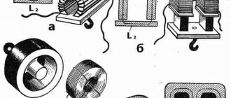
In Fig. Figure 9.12 schematically shows the magnetic systems of a magneto-electric measuring device (a) and a polarized relay (b). These systems, like most of their kind, have several sections: 1) made of hard magnetic material—permanent magnet 1; 2) made of soft magnetic material 2, which serves as a magnetic core, and an air gap 3, the shape and dimensions of which are determined by the design and purpose of the device. When calculating a magnetic circuit with a permanent magnet, it is necessary to determine the magnetic flux and induction in the air gap or, based on a given flux, to find the optimal dimensions of a permanent magnet (smallest volume and dimensions).
Demagnetization characteristics of permanent magnets
The values of residual magnetic induction Br and coercive force Hc characterize the material of a permanent magnet: the larger they are, the higher its quality. As is known, on the hysteresis loop Br corresponds to H = 0, and at B = 0 H = Hc. Rice. 9.12. Magnetic circuits with permanent magnets
Rice. 9.13. Characteristics of demagnetization of permanent magnets: 1 - ANKO-4; 2 - ANKO-2; Z-AN-2; 4 - steel with 30% CO
Intermediate magnetic states are determined by the part of the magnetic hysteresis loop lying in the second quarter - the demagnetization characteristic (Fig. 9.12). This characteristic is used in the calculation of permanent magnets. According to the law of total current, the sum of the magnetic voltages of the sections of the magnetic circuit (Fig. 9.12) is equal to zero, since there is no external magnetizing force (ampere-turns): where Um.t is the magnetic voltage of the permanent magnet; - the sum of the magnetic voltages of all sections of the magnetic circuit, including air gaps, but without a permanent magnet.
The left and right sides of equality (9.5) are related to magnetic induction and flux by certain dependencies: Фт(Uм.т) - demagnetization curve of a permanent magnet (the shape repeats the demagnetization curve of the material from which the permanent magnet is made); Фм(Uм.с) - magnetization curve of a part of the device structure made of soft magnetic material; Ф0(Uм0) - a straight line passing through the origin of coordinates and repeating the dependence on other scales
Parameters of magnetic circuits
As I have already said, many laws for electrical circuits also apply to magnetic circuits. To generalize these laws, it is necessary to introduce some parameters characterizing magnetic circuits. Let us imagine an inhomogeneous and unbranched magnetic circuit
Inhomogeneous and unbranched magnetic circuit.
This circuit consists of three sections of length l1, l2, l3, having a cross section S1, S2, S3, and the magnetic field is created by a current I flowing through a solenoid containing N turns. Since the magnetic field lines are mainly closed through the magnetic circuit, the magnetic flux Φ can be considered the same throughout the magnetic circuit and is determined by the following expression
where B is magnetic induction,
S is the cross-sectional area penetrated by the magnetic flux.
Thus, magnetic flux is an analogue of current strength in electrical circuits.
According to the law of total current and circulation of the magnetic induction vector, we create the equation
where B1, B2, B3 are respectively the magnetic induction in sections l1, l2, l3 of the magnetic circuit;
μ0 – magnetic constant, μ0 = 4π*10-7 H/m;
μ1, μ2, μ3 – respectively, the relative magnetic permeability of sections l1, l2, l3 of the core;
N – number of turns of wire;
I – current flowing through the wire.
When using ferromagnets, determining the relative magnetic permeability presents some difficulties, therefore, instead of magnetic induction in this law, magnetic field strength is used, therefore for a given magnetic circuit the law of total current can be represented as follows
Expressing magnetic induction in terms of magnetic flux, we obtain the following expression
where S1, S2, S3 are, respectively, the cross-sectional area of sections l1, l2, l3 of the magnetic circuit.
Thus, drawing an analogy with an electric circuit, we obtain the following parameters of the magnetic circuit
where Em is the magnetomotive force,
Rm – magnetic resistance of the circuit.
Therefore, the above expression can be represented by the following expression
where Rm1, Rm1, Rm1 are respectively the magnetic resistances of sections l1, l2, l3 of the magnetic circuit.
9.1.3. Properties of ferromagnetic materials
The magnetic state of any point in an isotropic medium, i.e. a medium with identical properties in all directions, is completely determined by the magnetic field strength vector H
and the magnetic induction vector
B
, which coincide with each other in direction.
The basic unit of magnetic induction in the SI system is called tesla (T): 1 T = 1 Wb/m2 = 1 V s/m2. This is the induction of such a uniform magnetic field in which the magnetic flux Ф
through a surface of 1 m2 perpendicular to the direction of the magnetic field lines is equal to one Weber (Wb).
In a vacuum, induction and magnetic field strength are related by a simple relationship: B = m0H, where m 0 = 4p·10-7 H/m is the magnetic constant. For ferromagnetic materials, the dependence of induction on the magnetic field strength B ( H )
in the general case nonlinear.
In order to experimentally study the magnetic properties of a ferromagnetic material, it is necessary to carry out all measurements on a sample in which the magnetic field is uniform. Such a sample can be a toroid made of the ferromagnetic material under study (Fig. 9.5), the length of the magnetic lines in which is much greater than its transverse dimensions (thin-walled toroid). On the toroid there is a uniformly wound winding with the number of turns w
.
We can assume that in a toroid made of ferromagnetic isotropic material with tightly wound turns, all magnetic lines are circles, and the vectors of magnetic field strength and induction are directed tangentially to the corresponding circle. So, in Fig. 9.5 shows the average magnetic line and vectors H
and
B
at one of its points.
When calculating the strength and induction of the magnetic field in a thin-walled toroid, we can assume that all magnetic lines have the same length, equal to the length of the middle line 2 p
r
.
Let us assume that the ferromagnetic material of the thin-walled toroid is completely demagnetized and the current I
there is none in the winding (
B
= 0 and
H
= 0).
If we now smoothly increase the direct current I
in the coil winding, then a magnetic field will arise in the ferromagnetic material, the intensity of which is determined by the total current law (9.1):
H
= Iw /2 p r .
(9.3)
Each tension value H
The magnetic field in a thin-walled toroid corresponds to a certain magnetization of the ferromagnetic material, and, consequently, to the corresponding value of magnetic
induction B.
If the initial magnetic state of the material of a thin-walled toroid is characterized by the values of H
= 0,
B
= 0, then with a smooth increase in current we obtain a nonlinear dependence
B( H),
which is called the initial magnetization curve (Fig. 9.5, dashed line).
Starting from certain values of
the magnetic field
H B
in a thin-walled ferromagnetic toroid practically stops increasing and remains equal to
B max
.
This region of the B( H)
is called the technical saturation region.
If, having reached saturation, we begin to smoothly reduce the direct current in the winding, i.e., reduce the field strength (9.3), then the induction will also begin to decrease. However, the dependence B( H)
no longer coincides with the initial magnetization curve.
By changing the direction of the current in the winding and increasing its value, we obtain a new section of the dependence B( H).
At significant negative values of the magnetic field strength, technical saturation of the ferromagnetic material will occur again.
If we now continue the experiment: first reduce the reverse current, then increase the forward current until saturation, etc., then after several magnetization reversal cycles a symmetrical curve will be obtained for the B( H)
(Fig. 9.5, solid line).
This closed cycle B( H)
is called the limiting static hysteresis loop (or limiting static hysteresis cycle) of a ferromagnetic material.
If during symmetric magnetization reversal the technical saturation region is not reached, then the symmetric B( H)
is called a symmetric partial hysteresis loop of the ferromagnetic material.
The statistical limit cycle of hysteresis of ferromagnetic materials is characterized by the following parameters:
NS
- coercive force,
V r
- residual induction and
k = Br / BH - l 0 Hc
- squareness coefficient.
According to the value of the parameter H with
limiting static hysteresis cycle, ferromagnetic materials are divided into groups:
1) magnetic materials with low values of coercive force ( H s
< 0.05…0.01 A/m) are called soft magnetic;
2) magnetic materials with large values of coercive force ( H s
> 20…30 kA/m) are called hard magnetic.
Hard magnetic materials are used for the manufacture of permanent magnets, and soft magnetic materials are used for the manufacture of magnetic cores of electrical devices operating in magnetization reversal mode in extreme or frequent cycles.
Soft magnetic materials, in turn, are divided into three types: magnetic materials with a rectangular limiting static hysteresis loop, in which the rectangularity coefficient k
> 0.95 (Fig. 9.6, a);
magnetic materials with a rounded limiting static hysteresis loop, in which the squareness coefficient is 0.4 < < k
<0.7 (Fig. 9.6, b);
magnetic materials with linear properties, in which the dependence B ( H )
is almost linear:
B = m r m 0 N
(Fig. 9.6, c), where
m r
is the relative magnetic permeability.
All types of magnetic characteristics of ferromagnetic materials can be obtained from samples made either from various ferromagnetic alloys or from ferromagnetic ceramics (ferrites). A valuable property of ferrites, in contrast to ferromagnetic alloys, is their high electrical resistivity.
Magnetic cores made of ferromagnetic materials with a rectangular limiting static hysteresis cycle are used in the random access memory of digital computers, magnetic amplifiers and other automation devices. Ferromagnetic materials with a rounded limiting static hysteresis cycle are used in the manufacture of magnetic cores of electrical machines and devices. The magnetic cores of these devices usually operate in magnetization reversal mode in symmetrical private cycles. In basic calculations of the magnetic circuits of such electrical devices, symmetrical partial cycles are replaced by the main magnetization curve of the ferromagnetic material, which is the geometric locus of the vertices of the symmetrical partial cycles of a thin-walled ferromagnetic toroid (Fig. 9.7), obtained with a low-frequency sinusoidal current in the winding.
Using the main magnetization curve of a ferromagnetic material, the dependence of the absolute magnetic permeability is determined
m a
=
m r m 0
=
B/N
(9.4)
from tension N
magnetic field, which is shown in Fig. 9.7 with a dashed line.
In Fig. Figure 9.8 shows the main magnetization curves of some electrical steels used in electrical machines, transformers and other devices, as well as cast iron and permalloy.
Ferromagnetic materials with linear properties are used to make sections of magnetic circuits for inductors of oscillatory circuits with high quality factor. Such circuits are used in various radio devices (receivers, transmitters), in small-sized communication antennas, etc.
If on a section of a magnetic circuit with cross-sectional area S
Since the magnetic field is non-uniform, calculations can often be made using the average value of induction
Вср = Ф/ S
and the intensity
Нср
on the average magnetic line.
For example, for a toroid with a rectangular cross-section, internal radius rt ,
external radius
r 2
and height
h
, made of a magnetic material with linear properties
B = m r m 0 H
at
m r
= const (Fig. 9.6, c),
Where
From the obtained expressions it follows that
In the future, to simplify calculations, we will not take into account the inhomogeneity of the magnetic field in the cross section of each section of the magnetic circuit, and we will assume that the field in each section is uniform and is determined by the values of intensity and induction on the average magnetic line.
Laws of magnetic circuit
As I wrote above, many laws of electrical circuits are also suitable for magnetic circuits. For example, Ohm's law for a magnetic circuit is as follows: magnetic flux Φ is directly proportional to the magnetomotive force Em and inversely proportional to the total resistance of the magnetic circuit Rm . And it is expressed by the following formula, also called Hopkinson’s formula
In addition to Ohm's law, Kirchhoff's rules apply to magnetic circuits. So Kirghoff’s first law for magnetic circuits is as follows: the algebraic sum of magnetic fluxes ∑Φ at a node of a magnetic circuit is equal to zero. To explain this rule, let us depict a branched magnetic circuit
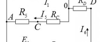
Branched magnetic circuit.
This magnetic circuit consists of two circuits ABCG and AGDE. The AG branch creates a magnetic flux Φ2, which at point A is divided into two fluxes Φ1 and Φ3. Thus, at point A the algebraic sum of magnetic fluxes is zero
Similarly, Kirchhoff's second law for a magnetic circuit sounds as follows: in the contour of a magnetic circuit, the algebraic sum of magnetomotive forces ∑Em is equal to the algebraic sum of magnetic stresses in individual sections.
The magnetic voltage on a section of the circuit is determined by the product of the magnetic flux Φ and the magnetic resistance of the section Rm, therefore, Kirchhoff’s second law will have the form
then for the magnetic circuit shown above, Kirchhoff’s second rule will have the form
Using these relationships, it is quite simple to calculate the required geometric dimensions of magnetic circuits for various magnetic systems, for example, transformers, chokes, inductors, and so on, which we will do below.
The formal analogy between electric and magnetic circuits indicated in the previous lecture allows us to extend all methods and techniques for calculating nonlinear resistive DC circuits to nonlinear magnetic circuits. In this case, for clarity, you can draw up an equivalent electrical equivalent circuit
the original magnetic circuit using which the calculation is performed.
The nonlinearity of magnetic circuits is determined by the nonlinear nature of the dependence, which is an analogue of the current-voltage characteristic and determined by the characteristics of the ferromagnetic material. When calculating magnetic circuits at constant fluxes, the basic magnetization curve is usually used. The loop-shaped nature of the dependence is taken into account when calculating permanent magnets and electrical devices based on them.
When calculating magnetic circuits in practice, two typical problems are encountered:
- the task of determining the magnitude of the magnetizing force (MF) required to create a given magnetic flux (given magnetic induction) on any section of the magnetic circuit ( synthesis problem
or
“direct” task
);
- the task of finding fluxes (magnetic induction) in individual sections of the circuit according to given NS values ( analysis task
or
“inverse” problem
).
It should be noted that problems of the second type are usually more complex and time-consuming to solve.
In general, depending on the type of problem being solved (“direct” or “inverse”), the solution can be carried out using the following methods:
-regular;
-graphic;
-iterative.
Moreover, when using each of these methods, it is initially necessary to indicate on the diagram the directions of the NS, if the directions of the currents in the windings are known, or to set them to positive directions if they need to be determined. Then the positive directions of magnetic fluxes are specified, after which you can proceed to drawing up an equivalent equivalent circuit and calculations.
Magnetic circuits according to their configuration can be divided into unbranched
and
branched.
In an unbranched magnetic circuit, the same flux occurs in all its sections, i.e. different sections of the circuit are connected to each other in series. Branched magnetic circuits contain two or more circuits.
Regular calculation methods
These methods solve problems of the first type - “direct” problems. In this case, the configuration and main geometric dimensions of the magnetic circuit, the magnetization curve (curves) of the ferromagnetic material and the magnetic flux or magnetic induction in any section of the magnetic circuit are given as the initial data for the calculation. It is required to find the NS, winding currents or, with known values of the latter, the number of turns.
1. Direct” problem for an unbranched magnetic circuit
Problems of this type are solved in the following sequence:
1. A middle line is outlined (see the dotted line in Fig. 1), which is then divided into sections with the same cross-section of the magnetic circuit.
2. Based on the constancy of the magnetic flux along the entire circuit, the induction values are determined for each section:
.
3. Using the magnetization curve for each value, the strengths in the ferromagnetic areas are found; The field strength in the air gap is determined according to
4. According to Kirchhoff’s second law for a magnetic circuit, the desired NS is determined by summing the magnetic voltage drops along the circuit:
,
where is the length of the air gap.
2. “Direct” problem for a branched magnetic circuit
The calculation of branched magnetic circuits is based on the combined application of Kirchhoff's first and second laws for magnetic circuits. The sequence of solving problems of this type generally corresponds to the algorithm considered above for solving the “direct” problem for an unbranched chain. In this case, to determine the magnetic fluxes in sections of the magnetic core for which the magnetic intensity is known or can be calculated based on Kirchhoff’s second law, the algorithm should be used
| By |
In other cases, unknown magnetic fluxes are determined based on Kirchhoff's first law for magnetic circuits.
As an example of the analysis of a branched magnetic circuit for a given geometry of the magnetic circuit in Fig. 2 and the characteristics of the ferromagnetic core, we determine the NS necessary to create induction in the air gap.
The algorithm for solving the problem is as follows:
1. We set the positive directions of magnetic fluxes in the magnetic cores (see Fig. 2).
2. We determine the tension in the air gap and, according to the dependence for, the value .
3. According to Kirchhoff’s second law for the right contour, we can write
where we find it and according to the dependence - .
4. In accordance with Kirchhoff's first law
.
Then, and from the dependence we determine .
5. In accordance with Kirchhoff’s second law, for the desired NS the following equation holds:
.
Graphical calculation methods
Problems of the second type—“inverse” problems—are solved using graphical methods. In this case, the configuration and geometric dimensions of the magnetic circuit, the magnetization curve (curves) of the ferromagnetic material, as well as the NS windings are specified as the initial data for the calculation. It is required to find the values of fluxes (inductions) in individual sections of the magnetic circuit.
These methods are based on a graphical representation of the Weber-ampere characteristics of linear and nonlinear sections of a magnetic circuit, followed by solving algebraic equations written according to Kirchhoff's laws using corresponding graphical constructions on a plane.
1. “Inverse” problem for an unbranched magnetic circuit
Problems of this type are solved in the following sequence:
1. They are specified by the flow values and the NS is determined for them, as when solving a “direct” problem. In this case, one should strive to select two sufficiently close flux values in order to obtain , somewhat less and slightly larger than the given value of NS.
2. Based on the data obtained, part of the characteristic of the magnetic circuit is constructed (near the given value of the NS), and from it the flux corresponding to the given value of the NS is determined.
When calculating unbranched magnetic circuits containing air gaps, it is convenient to use the intersection method, in which the desired solution is determined by the intersection point of the nonlinear Weber-ampere characteristic of the nonlinear part of the circuit and the linear characteristic of the linear section, constructed based on the equation
where is the magnetic resistance of the air gap.
2. “Inverse” problem for a branched magnetic circuit
Replacing the magnetic circuit with an equivalent electrical circuit (see Fig. 3, which shows the equivalent circuit of the magnetic circuit in Fig. 2) allows you to solve problems of this type using all the graphical methods and techniques used in the analysis of similar nonlinear DC electrical circuits.
In this case, when calculating magnetic circuits containing two nodes (a large number of magnetic circuits used in practice have this configuration), the two-node method is widely used. The idea of solving this method is similar to that considered for nonlinear resistive DC circuits and is as follows:
1. The dependences of the fluxes in all branches of the magnetic circuit are calculated as a function of the total value of the magnetic voltage between the nodes and .
2. It is determined at what point Kirchhoff’s first law is graphically implemented. The flows corresponding to this point are the solution to the problem.
Iterative calculation methods
These methods, the essence of which was discussed in the analysis of nonlinear resistive DC circuits, are approximate numerical methods for solving nonlinear algebraic equations that describe the state of a magnetic circuit. As noted above, they lend themselves well to machine algorithmization and are currently widely used in the study of complex magnetic circuits on digital computers. When analyzing relatively simple circuits containing a small number of nodes and nonlinear elements in an equivalent electrical equivalent circuit (usually up to two or three), it is possible to implement methods “manually”.
As an example, we present the algorithm for calculating the magnetic circuit in Fig. 1, in which, given the geometry of the magnetic core, the characteristics of the core material and the value of NS F, it is necessary to find the flux F.
In accordance with the step-by-step calculation for this circuit, we can write
| , | (1) |
Where .
We set the value, calculate for the th sections of the magnetic circuit, find from the magnetization curve, calculate and use (1) determine for the next approximation, etc., until the equality is satisfied with a given error.
Static and differential inductance of a coil with a ferromagnetic core
Let us have a coil with a ferromagnetic core, shown in Fig. 4.
According to the definition of flux linkage
| , | (2) |
and based on the law of total current, from where
| . | (3) |
From relations (2) and (3) it follows that the function qualitatively has the same form as . Thus, the dependences of relative magnetic permeability and inductance are also similar, i.e. presented in the previous lecture in Fig. 2 curves and are qualitatively similar to curves and .
Static inductance of a coil with a ferromagnetic core
;
differential inductance
.
If the magnetic conductivity of the core in Fig. 4 denote by , then and , from where
| (4) |
Using relation (4), we show the effect of the air gap on the inductance of the coil.
Let the coil in Fig. 4 has an air gap. Then the total magnetic resistance of the circuit
,
where
.
When , therefore
.
Thus, the air gap linearizes the coil with a ferromagnetic core. A gap for which the inequality holds is called a large gap.
Literature
- Fundamentals
of circuit theory: Textbook. for universities / G.V. Zeveke, P.A. Ionkin, A.V. Netushil, S.V. Strakhov. –5th ed., revised. –M.: Energoatomizdat, 1989. -528 p. - Bessonov L.A.
Theoretical foundations of electrical engineering: Electric circuits. Textbook for students of electrical engineering, energy and instrument engineering specialties of universities. –7th ed., revised. and additional –M.: Higher. school, 1978. –528 p. - Theoretical
foundations of electrical engineering. Textbook for universities. In three volumes. Under general. ed. K.M.Polivanova. T.2. Zhukhovitsky B.Ya., Negnevitsky I.B. Linear electrical circuits (continued). Nonlinear circuits. –M.: Energia- 1972. –200 p.
Test questions and tasks
- What two types of problems are encountered when calculating magnetic circuits? Give them a description.
- What methods exist for calculating magnetic circuits?
- What methods are used to solve “inverse” problems?
- How does the air gap affect the inductance of a nonlinear coil?
- What is a big gap?
- In the magnetic circuit in Fig. 2 are given and . Create an algorithm for calculating the length of the air gap.
- Create an algorithm for iterative calculation of the flux in the air gap of the magnetic circuit in Fig. 2 for a given NS.
- Write the law of electromagnetic induction using static and differential inductances.
Practical use
Ohm's formula is often used to answer the following questions:
- Calculation of magnetomotive force.
- Calculation of the number of turns of wire that, at a given current, will provide the required amount of magnetic flux.
As an example, consider the magnetic circuit shown in the figure below.
Let's agree that the first section is made of cast steel, the second is made of electrical steel, and the third is an air gap. It is required to determine the number of turns of the winding capable of providing a magnetic flux, which is equal to 0.0036 Weber for a current of 2 Amperes. Based on the dimensions indicated in the diagram, you can calculate the lengths of sections and cross-sectional areas of the part:
To find the value of magnetic induction, the data from the conditions of the problem should be substituted into the appropriate formula.
To find the magnitude of the magnetic field strength, you will need to open a graph of the relationship between magnetic induction and intensity in the reference book and determine what value corresponds to 1.5 Tesla. For cast steel this value is approximately 700 A/m, and for electrical steel - 3000 A/m. For an air gap, the desired value can be obtained by using the appropriate formula:
Using Ohm's law for a magnetic circuit, you can determine the number of turns by substituting the found values:
Therefore, in the case under consideration, 4083.5 turns will be required to provide the required parameters.
As we can see, when solving practical problems in electrical engineering, it is convenient to use concepts such as magnetomotive force and magnetic resistance.
It should also be said that without magnetic fluxes there would probably not have been such an industry as electrical engineering. After all, the properties of the magnetic field are the basis for the operation of many modern devices, including transformers, electric motors, generators, measuring instruments, and various sensors.
Magnetomotive force (MMF)
Main article: Magnetomotive force
Just as electromotive force (EMF) controls the flow of electric charge in electrical circuits, magnetomotive force (MMF) “controls” magnetic flux through magnetic circuits. The term magnetomotive force, however, is a misnomer because it is not a force or anything that moves. Perhaps it's better to just call it MMF. By analogy with the definition of EMF, the magnetomotive force F { Displaystyle { mathcal {F} }} around a closed loop is defined as:
F = ∮ HOUR ⋅ d l . { displaystyle { mathcal {F} } = oint mathbf {H} cdot mathrm {d} mathbf {l}.}
MMF represents the potential that a hypothetical magnetic charge would gain by completing a cycle. Controlled magnetic flux is no
magnetic charge current; it simply bears the same relation to MMF as electric current has to EMF. (See detailed description of microscopic sources of resistance below.)
The unit of magnetomotive force is the ampere-turn (At), represented by a steady direct electric current of one ampere flowing in a single-turn loop of electrically conductive material into a vacuum. Gilbert (Gb), established by IEC in 1930[1] This is the CGS unit of magnetomotive force and is a unit slightly smaller than the ampere-turn. The apartment is named after William Gilbert (1544–1603), an English physician and natural philosopher.
1 GB = 10 4 π V ≈ 0.795775 V { displaystyle { begin {align} 1 ; { text {Gb}} & = { frac {10} {4 pi}} ; { text {At}} & approximately 0.795775 ; { text {At}} end {align}}} [2]
Magnetomotive force can often be quickly calculated using Ampere's Law. For example, the magnetomotive force F { Displaystyle { mathcal {F} }} of a long coil is:
F = N i { displaystyle { mathcal {F} } = NI}
where N
this is the number of turns and
I
is the current in the coil.
In practice, this equation is used for the MMF of real inductors with N
being the winding number of the induction coil.
Applications
- Air gaps may be created in the cores of some transformers to reduce the effects of saturation. This increases the resistance of the magnetic circuit and allows it to store more energy before the core saturates. This effect is used in cathode ray tube video display flyback transformers and in some types of switching power supplies.
- Resistance variation is the principle behind the reluctance motor (or variable reluctance generator) and the Alexanderson Generator.
- Multimedia music speakers usually have magnetic shielding to reduce magnetic interference caused by televisions and other CRTs. The speaker magnet is coated with a material such as soft iron to minimize stray magnetic field.
Resistance can also be applied to variable reluctance (magnetic) pickups.
Circuit models
The most common way to represent a magnetic circuit is the resistance-resistance model, which draws an analogy between electrical and magnetic circuits. This model is good for systems containing only magnetic components, but for modeling a system containing both electrical and magnetic parts, it has serious shortcomings. It does not properly model power and energy flow between electrical and magnetic domains. This is because electrical resistance dissipates energy, while magnetic resistance stores it and returns it later. An alternative model that correctly models the energy flow is the gyrator-capacitor model.