In the course of general physics, Ohm's and Kirchhoff's laws, which include voltages, currents and resistances, are mainly used to calculate electrical circuits. However, to calculate complex electrical circuits, and especially AC circuits, it is advisable to use conductivity instead of resistance.
Conductivity in a DC circuit g is the reciprocal of resistance
The SI unit of conductivity is the siemens (in honor of the 19th century German electrical engineer E.W. Siemens).
1 Sim is the conductivity of a conductor with a resistance of 1 ohm.
In alternating current circuits, as is known, there are three types of resistance: active R, reactive and total g. By analogy with this, three types of conductances have been introduced: active g, reactive b and total y. However, only the admittance y is the reciprocal of the total resistance:
To introduce active g and reactive b conductivities, consider an alternating current circuit of active R and inductive reactances connected in series (Fig. 1-25, a). Let's construct a vector diagram for it (Fig. 1-25, b). We will decompose the current in the circuit into active and reactive components and from the resulting triangle of currents we will move on to the triangle of resistance (Fig. 1-25, c). From the latter we have:
From the vector diagram (see Fig. 1-25, b) taking into account formula (1.30) we have:
where is the active conductivity,
where is the reactivity.
Now let's establish the relationship between conductivities. For the circuit under consideration we have:
Substituting the values from relations (1.31) and (1.32) respectively, we obtain:
where is the total conductance of the circuit.
By analogy with the resistance triangle (Fig. 1-25, c), we build a conductivity triangle (Fig. 1-25, d). By analogy with inductive and capacitive reactance, a distinction is made between inductive and capacitive conductivity.
In the case of a branched circuit (Fig. 1-26, a), the circuit can be easily converted into a so-called equivalent circuit (Fig. 1-26, b), in which two branches are replaced by one with corresponding equivalent active and
reactances. Calculating the latter resistance, as well as other circuit parameters, is easier using conductances. Let us establish the basic laws for conductivity in a branched circuit.
Let us express the total current in terms of its components or equivalent conductivities:
In turn, the active component of the total current is equal to the sum of the active components of the branch currents:
i.e., the equivalent active conductance of the branch is equal to the arithmetic sum of the active conductances of the branches.
Since the reactive components of the branches of the circuit under consideration are in antiphase, then for the reactive component of the total current we have:
i.e., the equivalent reactive conductivity of the branching is equal to the algebraic sum of the reactive conductivities of parallel branches, and is taken with a “plus” sign, and with a “minus” sign.
. Capacitor (ideal capacity)
The processes for an ideal container are similar. Here . Therefore, from (3) it follows that. Thus, no active power is consumed in the inductor and capacitor (P = 0), since irreversible conversion of energy into other types of energy does not occur in them. Here only energy circulation occurs: electrical energy is stored in the magnetic field of a coil or the electric field of a capacitor for a quarter of a period, and over the next quarter of a period the energy is returned to the network. Because of this, the inductor and capacitor are called reactive elements, and their resistances X L and X C, in contrast to the active resistance R of the resistor, are called reactive.
The intensity of energy exchange is usually characterized by the highest value of the rate of energy input into the magnetic field of a coil or the electric field of a capacitor, which is called reactive power
.
In general, the expression for reactive power has the form:
It is positive when the current is lagging (inductive load -) and negative when the current is leading (capacitive load -). The unit of power as applied to the measurement of reactive power is called reactive volt-ampere
(VAR).
In particular, for the inductor we have: , since.
.
From the latter it can be seen that the reactive power for an ideal inductor is proportional to the frequency and the maximum energy reserve in the coil. Similarly, we can obtain for an ideal capacitor:
.
Resistor (ideal active resistance).
Here the voltage and current (see Fig. 2) are in phase, so the power is always positive, i.e. resistor consumes active power
Transient processes in linear electrical circuits. Basic concepts, laws of communication.
With all changes in the electrical circuit: switching on, switching off, short circuit, fluctuations in the value of any parameter, etc. – transient processes occur in it, which cannot occur instantly, since an instantaneous change in the energy stored in the electromagnetic field of the circuit is impossible. Thus, the transient process is caused by a discrepancy between the amount of stored energy in the magnetic field of the coil and the electric field of the capacitor and its value for the new state of the circuit. During transient processes, large overvoltages, overcurrents, and electromagnetic oscillations can occur, which can disrupt the operation of the device until it fails. On the other hand, transient processes find useful practical application, for example, in various types of electronic generators. All this necessitates the study of methods for analyzing non-stationary operating modes of a circuit.
Basic methods for analyzing transient processes in linear circuits:
- Classic method
consisting in the direct integration of differential equations describing the electromagnetic state of the circuit.
Operator method
which consists in solving a system of algebraic equations regarding images of the desired variables, followed by the transition from the found images to the originals.
Frequency method
based on the Fourier transform and widely used in solving synthesis problems.
Calculation method using the Duhamel integral,
used when the disturbance curve has a complex shape.
State variable method,
which is an ordered method for determining the electromagnetic state of a circuit based on solving a system of first-order differential equations written in normal form (Cauchy form).
Commutation laws
| Name of the law | Statement of the law |
| First law of commutation (law of conservation of flux linkage) | The magnetic flux coupled to the inductance coils of the circuit, at the moment of commutation, retains the value that it had before commutation, and begins to change precisely from this value: . |
| Second law of commutation (law of conservation of charge) | The electric charge on capacitors connected to any node, at the moment of switching, retains the value that it had before switching, and begins to change precisely from this value: . |
The laws of commutation can be proven by contradiction: if we assume the opposite, then we get infinitely large values of and, which leads to a violation of Kirchhoff’s laws.
In practice, with the exception of special cases (incorrect commutations), it is permissible to use these laws in a different formulation, namely:
first law of commutation -
in the branch with the inductor the current at the moment
.
second law of commutation –
voltage across the capacitor at the moment
commutation retains its pre-commutation value and subsequently begins to change from it: .
It must be emphasized that a more general formulation of the laws of commutation is the provision about the impossibility of abrupt changes at the moment of commutation for circuits with an inductor - flux linkages, and for circuits with capacitors - charges on them. As an illustration of what has been said, the diagrams in Fig. 2, transient processes in which refer to the so-called incorrect switchings
(the name comes from the neglect in such schemes of small parameters, the correct consideration of which can lead to a significant complication of the problem).
Indeed, when translated in the diagram in Fig. 2, and the switch from position 1 to position 2, the interpretation of the second law of commutation as the impossibility of an abrupt change in the voltage on the capacitor leads to failure of the second law of Kirchhoff. Similarly, when opening the key in the circuit in Fig. 2b, the interpretation of the first commutation law as the impossibility of an abrupt change in the current through the inductor leads to the failure of Kirchhoff's first law. For these circuits, based on the conservation of charge and, accordingly, flux linkage, we can write:
Dependent initial conditions are the values of the remaining currents and voltages, as well as derivatives of the desired function at the moment of switching, determined from independent initial conditions using equations compiled according to Kirchhoff's laws for. The required number of initial conditions is equal to the number of integration constants. Since it is rational to write an equation of the form (2) for a variable whose initial value refers to independent initial conditions, the problem of finding the initial conditions usually comes down to finding the values of this variable and its derivatives up to (n-1) order inclusive at.
Conductivity
When novice radio amateurs see an equation for calculating the total resistance of a parallel circuit, they naturally ask, “Where did that come from?” In this article we will try to answer this question.
Due to the fact that electrons, colliding with conductor particles, overcome some resistance to movement, it is customary to say that conductors have electrical resistance
.
Resistance is designated by the letter "R" and is measured in Ohms. However, any conductor can be characterized not only by its resistance, but also by the so-called conductivity
- the ability to conduct electric current. Conductivity is the reciprocal of resistance:
The greater the resistance, the less the conductivity and vice versa. Resistance and conductivity are opposite ways of referring to the same electrical property of materials. If, when comparing the resistances of two components, it turns out that the resistance of component "A" is half that of component "B", then we can alternatively express this relationship by saying that the conductivity of component "A" is twice the conductance of component "B". If the resistance of component "A" is one-third that of component "B", then component "A" can be said to be three times more conductive than component "B", and so on.
Conductivity is designated by the letter “G”, and its unit of measurement was originally “Mo”, that is, “Ohm” written backwards. But, despite the relevance of this unit, it was later replaced by “Siemens” (abbreviated as Sm or S).
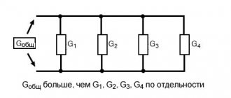
Now let's go back to our parallel circuit example. When viewed from a resistance perspective, having multiple paths (branches) for electron flow reduces the overall resistance of the circuit because it is easier for electrons to flow through multiple paths than through one path that has some resistance. If we consider a circuit from the point of view of conductivity, then multiple paths for the flow of electrons, on the contrary, increase the conductivity of the circuit.
The total resistance of a parallel circuit is less than any of its individual resistances because multiple parallel branches create less obstruction to the flow of electrons than each resistor individually:
The total conductivity of a parallel circuit is greater than the conductivity of any of its individual branches, since parallel-connected resistors conduct electric current better than each resistor individually:
It would be more accurate to say that the total conductivity of a parallel circuit is equal to the sum of its individual conductances:
Knowing that conductivity is equal to 1/R, we can transform this formula into the following form:
From this formula it can be seen that the total resistance of the parallel circuit will be equal to:
Well, we have found the answer to the question posed at the beginning of the article! You should be aware that conductivity is very rarely used in practice, and therefore this article is purely educational.
Short review:
- Conductivity is the opposite value of resistance.
- Conductivity is designated by the letter “G” and is measured in Mo or Siemens.
- Mathematically, conductivity is the inverse of resistance: G=1/R
Reactive conductivity is due to the presence of capacitance between phases and between phases and ground, since any pair of wires can be considered as a capacitor.
For overhead power lines, the value of linear reactive conductivity is calculated using the formulas:
7,58 ×10 — 6 b
0 р lg
D avg
.
R
pr eq
Cleavage increases b
0 at 21¸33%.
For CLEP, the value of linear conductivity is often calculated using the form
b
0 =
w
×
C
0 .
Capacitance size C
0 is given in the reference literature for various brands of cable.
The reactive conductivity of a network section is calculated using the formula:
B = b
0 ×
l
.
For overhead power lines the value b
0 is significantly less than that of cable power lines,
small, since D
av. overhead power lines >>
D
av. power transmission lines.
Under the influence of voltage, a capacitive current flows in the conductivities (bias current or charging current):
I
c =
V
×
U
f.
The magnitude of this current determines the loss of reactive power in reactive conductivity or the charging power of the power line:
D Q c
=
Q
charge = 3 ×
U
×
I c
=
B
×
U
2 .
In regional networks, charging currents are comparable to operating currents. At U
nom = 110 kV, the value of
Q
c is about 10% of the transmitted active power,
at U
rated = 220 kV –
Q
s
≈ 30%
R. Therefore, it must be taken into account in calculations. In a network with a rated voltage of up to 35 kV, the value of Qc
can be neglected.
Power line equivalent circuit
So, a power line is characterized by active resistance R
l, jet con-
x line
l, active conductivity
G
l, reactive conductivity
V
l. In calculations, power lines can be represented by symmetrical P- and T-shaped circuits (Fig. 4.6).
| R | X | R/2 X/2 | X/2 |
| R/2 | |||
| B /2 | G /2 | B /2 | |
| G | B | ||
| G/2 |
Figure 4.6 – Equivalent circuits for power lines: a) U-shaped; b) T-shaped
The U-shaped scheme is used more often.
Depending on the voltage class, certain parameters of the complete equivalent circuit can be neglected (see Fig. 4.7):
· Overhead power lines with voltage up to 110 kV (D R
core » 0);
· Overhead power lines with voltage up to 35 kV (D R
cor » 0, D
Q
c » 0);
· CLEP voltage 35 kV (reactance » 0)
· CLEP with voltage 20 kV (reactance » 0, dielectric losses » 0);
· CLEP with voltage up to 10 kV (reactance » 0, dielectric losses » 0, D Q
c » 0).
| X | R | X | R | |
| B /2 | B /2 | |||
| A) | b) | |||
| R | ||||
| R | R | |||
| G/2 | B/2 | B/2 | B/2 | B/2 |
| G/2 | ||||
| V) | G) | d) |
Figure 4.7 – Simplified power transmission line equivalent circuits:
a) overhead power lines at U
rated up to 110 kV;
b) overhead power lines at U
rated up to 35 kV;
c) CLEP at U
nom 35 kV;
d) CLEP at U
rated 20 kV;
e) CLEP at U
nom 6-10 kV;
Lecture No. 5
Transformer equivalent circuit parameters
13. General information.
14. Two-winding transformer.
15. Three-winding transformer.
16. Two-winding transformer with a split low-voltage winding.
17. Autotransformer.
General information
At power plants and substations, three-phase and single-phase, two-winding and three-winding power transformers and autotransformers, and single-phase and three-phase power transformers with a split low-voltage winding are installed.
The transformer abbreviation contains the following information sequentially (from left to right):
type of device ( A
– autotransformer, without designation – transformer);
number of phases ( O
– single-phase,
T
– three-phase);
· presence of a split low voltage winding – P
;
· cooling system ( M
– natural circulation of oil and air,
D
– forced air circulation and natural circulation of oil,
MC
– natural circulation of air and forced circulation of oil,
DC
– forced circulation of air and oil, etc.);
· number of windings (without designation - two-winding, T
– three-winding-precise);
· presence of a voltage regulation device under load (OLTC);
· execution ( Z
– protective,
G
– lightning-resistant,
U
– improved,
L
– with cast insulation);
· specific area of application ( C
– for auxiliary systems of power plants,
F
– for electrification of railways);
· rated power in kVA∙A,
· winding voltage class (network voltage to which the transformer is connected) in kV.
Double winding transformer
In electrical diagrams, a two-winding transformer is represented as follows (Fig. 5.1):
| The windings indicate the circuit diagrams | |
| VN | connection of windings (star, star with well- |
| lem, triangle) and operating mode | |
| trawl: | |
| · star – with an isolated neutral | |
| NN | I pour; |
| · star with zero – there is a connection | |
| neutral to ground. | |
| Figure 5.1 – Conventional image | In accordance with the adopted system |
| two-winding | my notation is abbreviation trans- |
| transformer. | |
| formator TDN-10000/110/10 decoding | |
| is converted: three-phase transformer |
ny, two-winding with forced air circulation and natural oil circulation and a voltage regulation system under load. Rated power – 10000 kV∙A, voltage class of the high voltage winding
– 110 kV, low voltage – 10 kV.
In practical calculations, a two-winding transformer is most often represented by an L-shaped equivalent circuit (Fig. 5.2).
| U 1 | R t | X t | U 2 * |
| In t | G t |
Figure 5.2 – L-shaped equivalent circuit of a two-winding transformer
X
t =
X
in +
X
n *.
The active and reactive resistance of the transformer (longitudinal branch) is the sum of the active and reactive resistance of the high-voltage winding and the low-voltage winding reduced to it:
R
t =
R
in +
R
n *;
The transverse branch of the equivalent circuit is represented by active G
t and reactive
Vt
conductivities. Conductivity is usually connected from the side of the primary winding: for step-up transformers - from the side of the low voltage winding, for step-down transformers - from the side of the high voltage winding.
In such an equivalent circuit there is no transformation, that is, there is no ideal transformer. Therefore, in the calculations the secondary voltage U
2 * turns out to be reduced to the voltage of the primary winding.
Active conductivity is caused by active power losses in the transformer steel due to magnetization reversal and eddy currents, reactive conductivity
– magnetizing power. In calculations of electrical network modes, conductivities are replaced by a load equal to no-load losses.
The parameters of the transformer equivalent circuit are determined from two experiments
– idle and short circuit. In the experiments, the following values are determined, which are indicated in the transformer’s passport data:
active power loss in idle mode D P
x in kW;
active power loss in short circuit mode D P
k in kW;
short circuit voltage U
k, in %;
no-load current I
x, in %.
The values of active and reactive resistance are found from short circuit experience (Fig. 5.3). The experiment is performed as follows: the low-voltage winding is short-circuited, and the same voltage ( U
j) so that the rated current flows in both.
| So | How | voltage |
| I 1nom | short | closures |
| I 2nom | much | less nominal |
| U to | cash | voltage |
| transformer, then the heat- | ||
| ri active power in | ||
| conductivity | practically | |
| skis are zero. So | ||
| Figure 5.3 – Short circuit experience | way, | all losses |
| power in operating mode | ||
| two-winding transformer. | ||
| me short | closures | |
| go to heat the windings. Mathematically this can be written: | ||
| D P =3× I 2 | × R . | (5.1) |
| To | 1nom | T |
If in formula (5.1) the current value is written in terms of the power and rated voltage of the high voltage winding
Short circuit voltage U
k consists of the voltage drop across the active
U
k a and reactive
U
k p resistances. Let's express them as a percentage of the rated voltage.
Voltage drop in the active resistance of the transformer:
| U | to a | 3 ×I | ×R | ||
| U | , % = | ×100 = | 1nom | T | ×100. |
| to a | U in nom | U in nom |
R into the expression
t. We get:
| ×D P × U 2 | |||||||||
| 3 ×I | ×R | 3 ×I | D P | ||||||
| U | , % = | 1nom | T | ×100 | = | 1 room per room | ×100 = | To | ×100. |
| to a | |||||||||
| U in nom | U in nom × S nom 2 | S nom |
Thus, the magnitude of the voltage drop in the active resistance, expressed as a percentage, is proportional to the active power losses in short-circuit mode.
The expression for the voltage drop in reactance in percent is as follows:
| U to p | |||||
| 3 ×I | ×X | T | |||
| U | , % = | ×100 = | 1nom | ×100. | (5.2) |
| k p | U in nom | U in nom |
From it we can find the value of the reactance of the transformer:
| X t = | U cr × U in nom | . |
| × | 3 × I 1 nom |
Multiply and divide the resulting expression by U
in nom:
| X t = | U cr × U in nom | × | U in nom | = | U cr × U in 2 nom | . |
| U in nom | 100 × S nom | |||||
| × 3 | × I 1 nom |
In modern transformers, active resistance is much greater than reactive resistance. Therefore, in practical calculations it can be assumed that U
k r ≈
U
k. Then, the formula for calculating the inductive reactance of a transformer has the form:
| X | = | U to × U to 2 | nom | . |
| T | ||||
| × S nom |
Transformers have voltage regulation devices (on-load tap-changer or tap-changer), which allow changing transformation ratios. Therefore,
rank U
k (hence, the magnitude of the inductive reactance) depends on the branching of the on-load tap-changer or tap-changer devices. In calculations of steady-state conditions, this dependence is neglected. It is taken into account when calculating short-circuit currents when choosing automation and relay protection devices.
The conductivities of the magnetization branch are determined from the no-load test (Fig. 5.4), which is performed at rated voltage. In this mode, the transformer consumes power equal to the no-load losses:
I
2 = 0
Figure 5.4 – Experience of no-load operation of a two-winding transformer.
| G | = | D P x | . |
| T | |||
| U in 2 | |||
| nom |
D S
x = D
P
x +
j
D
Q
x.
Active power losses are proportional to the active conductivity of the transformers
D P
x =
U
in 2 nom ×
G
t.
From here the amount of active conductivity can be determined
Reactive power losses are proportional to the reactive conductivity of the transformer:
D Q
x =
U
in 2 nom ×
B
t.
Therefore, the value of the reactive conductivity of the transformer is equal to:
B
t = D
Q
x.
U
in 2 rooms
The amount of reactive power loss is proportional to the magnetizing current
| D Q x =3× I m × U in nom f, | (5.3) |
where U
nom f – phase rated voltage of the transformer.
The magnitude of the no-load current is the sum of the magnetizing current I
μ and then in steel
I
steel:
I
x=
I
μ+
I
steel.
Since the current value in steel is about 10% of the magnetization current, expression (5.3) can be written:
D Q
x »3×
I
x ×
U
in nom f.
In the passport data, the no-load current value is given as a percentage of the rated current. Therefore we can write:
Taking into account the obtained expression, the formula for calculating reactive conductivity has the form:
B
t =
I
x % × ×
S
nom.
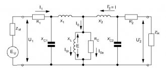
In Fig. 14.14, and the same circuit elements that were considered are connected in parallel (see Fig. 14.7, a). Let us assume that for this circuit the voltage u = U m sinωt
. and parameters of the circuit elements R, L, C. It is required to find the currents in the circuit and power.
Active resistance of wires and cables
It is known from electrical engineering that the total resistance under equal conditions to alternating and direct current will differ. This also applies to wires and cables. This is due to the fact that the alternating current is distributed unevenly across the cross section (surface effect). However, for wires made of non-ferrous metals and with an alternating voltage frequency of 50 Hz, this effect does not have too much influence and can be neglected. Thus, when calculating conductors made of non-ferrous metals, their resistance to alternating and direct current is assumed to be equal.
In practice, the active resistance of copper and aluminum conductors is calculated using the formula:
Where: l is the length in km, γ is the specific conductivity of the wire material m/ohm∙mm2, r0 is the active resistance of 1 km of wire per phase Ohm/km, s is the cross-sectional area, mm2.
The value of r0 is usually taken from reference tables.
The active resistance of the wire is also affected by the ambient temperature. The value of r0 at temperature Θ can be determined by the formula:
Where: α – temperature coefficient of resistance; r20 – active resistance at a temperature of 20 0С, γ20 – specific conductivity at a temperature of 20 0С.
Steel wires have significantly higher active resistance than similar wires made of non-ferrous metals. Its increase is due to a significantly lower specific conductivity and the surface effect, which is much more pronounced in steel wires than in aluminum or copper. Moreover, in steel wires there are losses of active energy due to eddy currents and magnetization reversal, which is taken into account in equivalent circuits of lines as an additional component of active resistance.
The active resistance of steel wires (unlike wires made of non-ferrous metals) strongly depends on the amount of current flowing, so it is impossible to use a constant value of specific conductivity in calculations.
It is very difficult to analytically express the active resistance of steel wires depending on the flowing current, so special tables are used to determine it.
Vector diagram for a circuit with parallel connections of branches. Vector diagram method
For instantaneous quantities, in accordance with Kirchhoff’s first law, the current equation
Representing the current in each branch as the sum of the active and reactive components, we obtain
For effective currents you need to write a vector equation
The numerical values of the current vectors are determined by the product of the voltage and conductivity of the corresponding branch.
In Fig. 14.14, b a vector diagram corresponding to this equation is constructed. As usual when calculating circuits with parallel
connections of branches, vector
U is taken as the initial vector,
and then the current vectors in each branch are plotted, and their directions relative to the voltage vector are chosen in accordance with the nature of the conductivity of the branches. The starting point when constructing a current diagram is the point coinciding with the beginning of the voltage vector. From this point the vector l 1a of the active current
of branch
I
(in phase with the voltage), and from its end the vector
I 1p
of the reactive current of the same branch is drawn (leads the voltage by 90°).
These two vectors are components of the vector I 1 of the first branch current
.
Next, the current vectors of other branches are plotted in the same order. It should be noted that the conductivity of branch 3-3 is active
, therefore the reactive component of the current in this branch is zero.
In branches 4-4 and 5-5, the conductivities are reactive
, therefore there are no active components in the composition of these currents.
Inductive reactance of wires and cables
To determine the inductive reactance (denoted by X) of a cable or overhead line of a certain length in kilometers, it is convenient to use the expression:
Where: X0 is the inductive reactance of one kilometer of wire or cable per phase, Ohm/km.
X of one kilometer of overhead or cable line can be determined by the formula:
Where: Dav – average distance between wires or centers of cable cores, mm; d – diameter of the current-carrying cable core or wire diameter, mm; μt – relative magnetic permeability of the wire material;
The first term on the right side of the equation is due to the external magnetic field and is called external inductive reactance X0/. From this expression it is clear that X0/ depends only on the distance between the wires and their diameter, and since the distance between the wires is selected based on the rated line voltage, accordingly X0/ will increase with increasing rated line voltage. X0/ there are more overhead lines than cable lines. This is due to the fact that the current-carrying wires of the cable are located much closer to each other than the wires of overhead lines.
For one phase:
Where: D1:2 is the distance between the wires.
For a single three-phase line with wires arranged in a triangle:
When the wires of a three-phase line are located horizontally or vertically in the same plane:
An increase in the cross-section of the line wires leads to a slight decrease in X0/.
The second term in the equation for determining X0 is due to the magnetic field inside the conductor. It expresses the internal inductive reactance X0//.
Thus, the expression for X0 can be represented as:
For lines made of non-magnetic materials μ = 1, the internal inductive reactance X0// compared to the external X0/ is negligible, so it is very often neglected.
In this case, the formula for determining X0 will take the form:
For practical calculations, the inductive resistance of cables and wires is determined using the corresponding tables.
In the case of approximate calculations, it can be considered that for overhead lines with a voltage of 6-10 kV X0 = 0.3 - 0.4 Ohm/km, and for cable lines X0 = 0.08 Ohm/km.
The internal inductive reactance of steel wires is very different from X0// wires made of non-ferrous metals. This is due to the fact that X0// is proportional to the magnetic permeability μr, which strongly depends on the magnitude of the current in the wire. If for wires made of non-ferrous metals μr = 1, then for steel wires μr can reach a value of 103 and even higher.
X0// for lines laid with steel wires cannot be neglected. As a rule, this value is taken from tables compiled on the basis of experimental data.
Resistances r0 and X0// at certain current values can reach maximum values, and then decrease with increasing current. This phenomenon is explained by the magnetic saturation of steel.
Calculation formulas for a circuit with parallel connections of branches. Vector diagram method
From a vector diagram
it can be seen that all the active components of the current vectors are directed in the same way - parallel to the voltage vector, so their vector addition can be replaced with arithmetic ones to find the active component of the total current:
I a = I 1a + I 2a + I 3a
.
Reactive components
current vectors are perpendicular to the voltage vector, with inductive currents directed in one direction, and capacitive currents in the other.
Therefore, the reactive component of the total current in the circuit is determined by their algebraic sum, in which inductive currents are considered positive and capacitive currents are considered negative: I p = - I 1p + I 2p - I 4p + I 5p
.
The active, reactive and total current vectors of the entire circuit form a right triangle, from which it follows
Attention should be paid to possible errors when determining the total conductivity of a circuit from the known conductivities of individual branches:
it is impossible
to add arithmetically the conductivities of the branches if the currents in them are out of phase.
Full conductivity
circuits are generally defined as the hypotenuse of a right triangle, the legs of which are the active and reactive conductivities of the entire circuit expressed on a certain scale:
From the current triangle you can also go to the power triangle and to determine the power you can obtain the already known formulas
Active power
circuits can be represented as the arithmetic sum of the active powers of the branches.
Reactive power
chain is equal to the algebraic sum of the powers of the branches. In this case, the inductive power is taken to be positive, and the capacitive power to be negative: