Theoretical foundations of electrical engineering (TOE) is an engineering discipline that studies the laws of the theory of electricity and electromagnetism. The TOE course consists of two parts:
- theory of electrical circuits
- field theory
Get a solution on TOE
The study of TOE is the basis for understanding electrical engineering, automation, energy, instrument engineering, microelectronics, radio engineering and other subjects.
- Lectures on electrical engineering (TOE)
- Solving problems, tests and coursework
The purpose of studying the discipline “Fundamentals of Electrical Engineering and Electronics” is for the student to acquire an integral part of the complex of knowledge on electrical equipment and power supply of enterprises, which can be used in future professional activities.
General Electrical Engineering
When studying the discipline “TOE”, the student is provided with fundamental training in the field of general electrical engineering and electronics; connection is maintained with the disciplines of “mathematics”, “physics” and “chemistry” and continuity in the use of computers in the educational process, familiarization with the core problems of receiving, transmitting and converting electrical energy, basic provisions on electric drives and modern electronic base used in automatic circuits management, skills and concepts of professional terminology, mandatory for the solid mastery of subsequent disciplines and the practical use of acquired knowledge in solving professional problems.
Contents of the TOE course
- Basic terms and definitions of electrical engineering
- Electrical circuit
- Linear DC electrical circuits
- Calculation of an electrical circuit using the equivalent transformation method
- Calculation of an electrical circuit according to Kirchhoff's law
- Calculation of an electrical circuit using the loop current method
- Calculation of an electrical circuit using the superposition method
- Two node method
- Electric circuit power balance
- Potential Diagram Calculation
- Linear electrical circuits of single-phase sinusoidal alternating current
- Calculation of AC electrical circuits
- Algebraic operations with complex numbers
- Analysis of the electrical state of an AC circuit
- Analysis of a circuit with a resistive element
- Analysis of a circuit with an inductor
- Analysis of a circuit with a capacitor
- Circuit analysis with series connection of elements R, L, C
- Sinusoidal current circuit power
- Power factor and its economic significance
- Resonance in AC circuits
- Characteristic Features of Voltage Resonance
- Three-phase circuit power
- Calculation of three-phase circuits
- Single-phase transformers
- Three-phase transformers
- The principle of self-excitation of a parallel excitation DC generator
- Generator self-excitation conditions
- Operating principle of a DC motor
- Methods of speed control
- Methods for starting the engine
- Operating principle of an asynchronous motor
- Features of starting asynchronous motors
- Operating principle of a synchronous generator
- Operating principle of a synchronous motor
- Features of starting a synchronous motor
Lectures on TOE / LECTURE2
1.2.1 Kirchhoff's laws
Kirchhoff's laws are fundamental in circuit theory. First Law
- Kirchhoff's current law (KLC)
is formulated in relation to the nodes of an electrical circuit and reflects the fact that charges cannot accumulate in the nodes
.
It says: the algebraic sum of the currents of the branches converging at any node of the electrical circuit is equal to zero . Formally, this is written as follows:
, (2.1)
where m
— the number of branches converging at a node.
In this equation , currents that are equally oriented relative to a node have the same signs.
For example, the signs of outgoing currents can be considered positive, and those of incoming currents can be considered negative
.
The number of independent equations compiled according to the ZTK is equal to the number of independent nodes of the electrical circuit.
Second Law
-
Kirchhoff's stress law
(KLS)
is formulated in relation to circuits
and states:
the algebraic sum of the voltages of the branches in any circuit circuit is equal to zero .
, (2.2)
where n
— the number of branches included in the circuit.
In this equation , voltages that coincide with the direction of bypassing the circuit are written with a “+” sign, and those that do not coincide with a “-” sign.
Illustration of Kirchhoff's laws
Let's consider an example in which the currents of the branches of the resistive circuit shown in Fig. are calculated. 2.1, according to the method of Kirchhoff equations. The circuit has n y = 4 nodes, n b = 6 branches. Let's choose node 4 as the base one and compose n y - 1 = 3 equations according to the ZTK: for the 1st node -i 1 + i 3 + i 4 = 0; for the 2nd node -i 2 - i 3 + i 5 = 0; for the 3rd node i 2 - i 4 + i 6 = 0. Using the LNC we compose n in - n y + 1 = 3 equations for the circuits shown in the figure with arrows: for the 1st circuit -u r1 + u 1 + u 3 + u 5 = 0; for the 2nd circuit u r2 + u 2 - u 3 + u 4 = 0; for the 3rd circuit -u g2 - u 2 + u 6 - u 5 = 0. Or taking into account Ohm's law:
Figure 2.1 - Scheme reflecting the use of ZTK and ZNK
-u r 1 +R 1 i 1 + R 3 i 3 + R 5 i 5 = 0 ;
u g 2 + R 2 i 2 - R 3 i 3 + R 4 i 4 = 0;
- u r2 - R 2 i 2 + R 6 i 6 - R 5 i 5 = 0.
By solving these systems of equations together, the required currents are found.
1.2.2 Conversion of electrical circuits
Transformations of electrical circuits are used to simplify calculations.
The most typical conversion methods are as follows.
Series connection of elements.
According to the ZTK,
when elements are connected in series, the same current flows through them
(Figure 2.2).
Figure 2.2 - Series connection of elements
According to the ZNK , the voltage applied to the entire circuit
:
. (2.3)
Then for a series connection of resistive elements
R1, R2, …, Rn we will have:
. (2.4)
For series connection of inductive elements
(Figure 2.2):
. (2.5)
For series connection of capacitive elements
:
. (2.6)
Thus
,
a circuit of n series-connected resistive, inductive or capacitive elements can be replaced by one equivalent resistive, inductive or capacitive element
.
Moreover, when finding the equivalent resistance or equivalent inductance, it is necessary to sum up the resistances and inductances of individual resistive and inductive elements, and to find the equivalent reciprocal capacitance, sum up the reciprocal values of the capacitances of individual capacitive elements
. For n = 2:
C = C1C2/(C1 + C2). (2.7)
When independent
voltage sources
, they
are replaced by one equivalent voltage source
with a reference voltage
u g equal to the algebraic sum of the reference voltages of the individual sources
.
Moreover, with the “+” sign we take the reference voltages that coincide with the reference voltage of the equivalent source,
and with the “-” sign - those that do not coincide (Figure 2.3).
Figure 2.3 - Series connection of voltage sources
Parallel connection of elements.
When
connecting elements in parallel
according to the code of conduct,
the same voltage will be applied to them
(Figure 2.4).
According to the ZTK, for the current of each of the circuits
shown in Figure 2.4,
we can write
:
. (2.8)
Figure 2.4 - Parallel connection of passive elements
Based on this equation for parallel connection of resistive elements
we get:
. (2.9)
For parallel connection of capacitive elements
:
. (2.10)
For parallel connection of inductive
elements:
. (2.11)
Hence
, a circuit
of n parallel-connected resistive, inductive or capacitive elements can be replaced by one equivalent
resistive, inductive or capacitive
element
.
Thus
,
when
connecting resistive, capacitive and inductive elements in parallel, to find the equivalent
conductivity and capacitance, the conductivity circuits or capacitances of the individual elements are added up
.
The equivalent reverse inductance
of the circuit
is found by summing the reverse inductances
of the individual inductive elements. In particular, for n = 2:
R = R1R2/(R1 + R2); L = L1L2/(L1 + L2) . (2.12)
Parallel-connected independent
current sources
can
be replaced by one equivalent current source with a driving current equal to the algebraic sum of the driving currents of the individual sources
.
Moreover, with the “+” sign we take the driving currents that coincide in direction with the driving current of the equivalent source
, and with the “-” sign - those that do not coincide (Figure 2.5).
Figure 2.5 - Parallel connection of current sources
When calculating electrical circuits, there is often a need to convert a voltage source with parameters
u g and R g into an equivalent current source with parameters i g and G g
, or vice versa - convert a current source into an equivalent voltage source.
These transformations are carried out in accordance with the formulas
ig = ug/Rg; Gg = 1/Rg. (2.13)
An example of
a star-delta conversion. In addition to series and parallel connections of elements, triangle and star connections of elements are very common (Figure 2.6).
Figure 2.6 - Delta and star connections
There are formulas for converting a
triangle connection into a star :
; ; . (2.14)
The reverse transition can be obtained using the formulas obtained from the previous ones:
R 12
= R 1 + R 2 + R 1 R 2 / R 3 ; R 23 = R 2 + R 3 + R 2 R 3 / R 1 ; R 31 = R 3 + R 1 + R 3 R 1 / R 2 .
(2.15) Similarly, there are formulas for the star-delta conversion of inductive and capacitive elements [1, p. 23-24].
1.2.3 Overlay principle
The principle of superposition
is of utmost importance in the theory of linear electrical circuits.
The overwhelming number of methods for analyzing linear circuits are based on this principle. If we consider the voltages and currents of the sources as setting influences, and the voltage and currents in individual branches of the circuit as the reaction (response) of the circuit to these influences, then the principle of superposition can be formulated as follows: the reaction of a linear circuit to the sum of influences is equal to the sum of reactions from each individual influence .
The principle of superposition
can be used
to find a reaction
in a linear chain
, either
under the influence of several sources
,
or under the complex arbitrary influence of a single source
.
Let us consider the case when several sources operate in a linear circuit.
In accordance
with the principle of superposition, to find the current i or voltage u in a given branch, we will alternately influence each source and find the corresponding partial reactions i k and u k to these influences
. Then the resulting reaction is determined as
, (2.16)
where n
— total number of sources.
Let us illustrate the principle of superposition (superposition) using the example of a resistive circuit shown in Figure 2.7, a.
Figure 2.7 - Illustration of the principle of superposition
Let's find the current in the resistive element R 3 . Let us first that there is only one source u r1 : the second voltage source is excluded and its terminals are short-circuited. In this case, we obtain a partial diagram shown in Figure 2.7b. Let us determine the current i 3 ' from the influence of voltage u g1 , taking into account that and :
. (2.17)
Now we assume that u r2 acts in the circuit . By excluding the source u r1 , we obtain the second partial circuit . The current i 3 " from the influence u r2 will be determined as, taking into account that and :
. (2.18)
We find the resulting current i 3 as an algebraic sum of partial currents : i 3 = i 3 ' + i 3 " . When determining the resulting currents, the “+” sign is taken for partial currents that coincide with the selected positive direction of the resulting current, and the “-” sign for those that do not coincide. As follows from the considered example, when drawing up partial electrical circuits, the excluded ideal voltage sources are short-circuited
.
If the
circuit contains voltage sources with internal resistances Rg
, when they are removed
their internal resistances Rg . In the presence of ideal current sources, the corresponding branches of the excluded sources are opened
, and in the presence of real sources they are replaced by their internal conductivities Gg.
If
of a complex shape is applied to a linear circuit , the application of the principle of superposition allows us to decompose this effect into the sum of the simplest ones
and
find the reaction of the circuit to each
of them separately
, followed by superimposing the results obtained
.
Methods of loop currents, nodal voltages and equivalent generator
Electronics
Mastering the electronics course includes lectures and practical exercises in solving problems. The course provides for the implementation of a cycle of independent calculation and graphic works with their subsequent defense upon delivery. Organizing and carrying out such work requires the development of a series of tasks on topics, as well as guidelines for solving standard tasks. Some typical calculations, for example, the calculation of complex circuits, involve quite large amounts of calculations, so it is advisable to use specialized mathematical programs for computer calculations.
Contents of the course “Fundamentals of Electronics”
- Basic semiconductor devices and elements
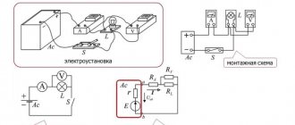
- Electrical measurements and instruments
- Types and methods of electrical measurements
- Errors of electrical measuring instruments
- Classification of electrical measuring instruments
- Characteristics of measuring instrument scales
- AC and DC current measurement
- DC and AC voltage measurement
- Power measurement in DC circuits
- Power measurement in single-phase AC circuits
- Power measurement in three-phase circuits
- Digital meters